calendar_todayarticle
3220 words
access_time
27 min
replay Modified
Table of Contents
Postulates of Ray Optics
Basic Postulates
Light travels in the form of rays
Optical media are characterized by their refractive index $n = c_0 / c$ with the time taken to travel a distance $d = nd / c_0$
The quantity $nd$ is the optical pathlength and is directly proportional to the time taken
Inhomogeneous media have $n(\bf{r})$ and the optical pathlength between $A$ and $B$ is therefore $\int_{A}^{B} n(\bf{r}) \ \mathrm{d}s$
Definition(Fermat’s Principle).
Optical rays travel along the path of least time.
$$\delta \int_{A}^{B} n (\bf{r}) \ \mathrm{d}s = 0$$
where $\delta$ is “the variation of” and signifies the optical pathlength is a point of inflection/minima/maxima (almost always a minima)
If there is a tie between many minimum-time paths, the rays take all paths simultaneously
Homogeneous Media
Rays travel in straight lines
Definition(Hero’s Principle).
In a homogeneous medium, the minimum-time path (required by Fermat’s Principle) is also the path of minimum distance
Reflection from a Mirror
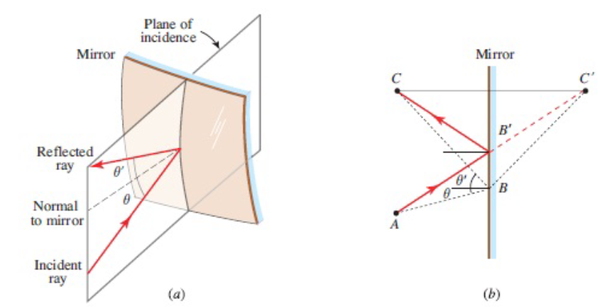
Definition(Law of Reflection).
Reflected rays lie in the plane of incidence
The angle of reflection $\theta’$ equals the angle of incidence $\theta$
Proof.
We will show that $\overline{AB} + \overline{BC}$ is the shortest possible path by Hero’s Principle.
Observe that $\overline{BC} = \overline{BC’}$; therefore, $\overline{AB} + \overline{BC’}$ must also be the shortest length. By coinciding $B$ with $B’$, we can see a straight line $\overline{AB’C’}$ connecting $A$ to $C’$.
Thus, $\overline{AB} + \overline{BC}$ is the shortest path and $\theta = \theta’$.
Refraction Between Media
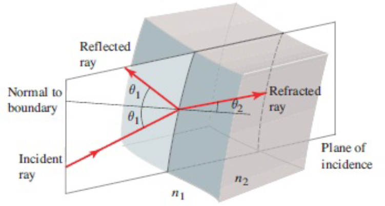
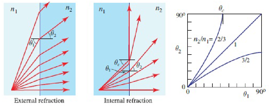
At the boundary between two media, an incident ray is split into two
The angle of incidence $\theta_1$ and angle of refraction $\theta_2$ are related by Snell’s Law
- Linear (small-angle) approximation: $n_1 \theta_{1} \approx n_{2} \theta_{2} \implies \theta_{2} \approx \left(\frac{n_{1}}{n_{2}}\right)\theta_{1}$
A third angle, the angle of deviation, represents the difference between the angles of incidence and refraction[Course handout, Introduction to Ophthalmic Optics, p. 15]
- Since it lies between $\theta_{1}$ and $\theta_{2}$, $\theta_{d} \coloneqq \theta_{1} - \theta_{2}$
Simple Optical Components
Mirrors
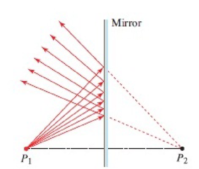
Reflects rays originating from the front of the mirror (i.e., $P_1$) such that the reflected ray forms a directed line segment with a collinear point behind the mirror (i.e., $P_2$)
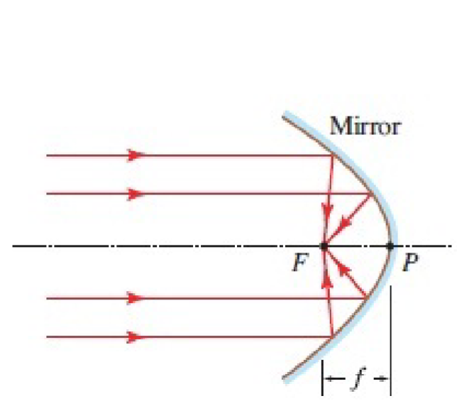
The surface of this mirror is a paraboloid
Focuses rays that are parallel to its axis at a single point, called the focus
The distance from the vertex to the focus is the focal length
Can be used as a collimator
A point source/beam with divergent rays is placed near the focus of a paraboloidal mirror, which causes the rays to become parallel and form a straight line by the Law of Reflection
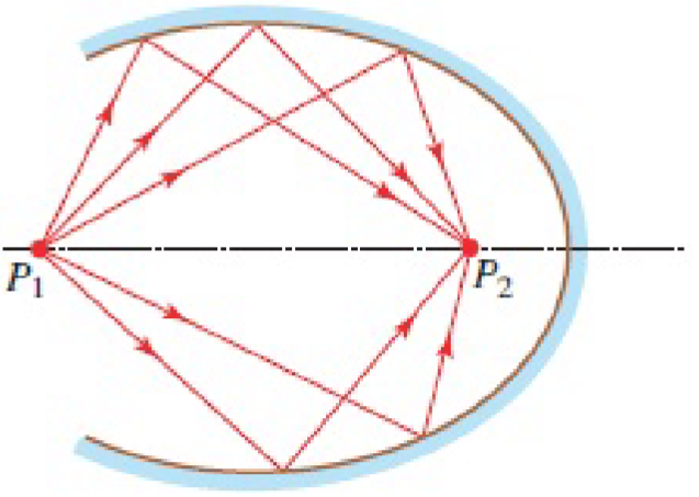
Reflects all rays originating from one focus, $P_1$, into the other focus, $P_2$
All paths taken from $P_1$ to $P_2$ are the same distance and thus taken simultaneously by Hero’s Principle
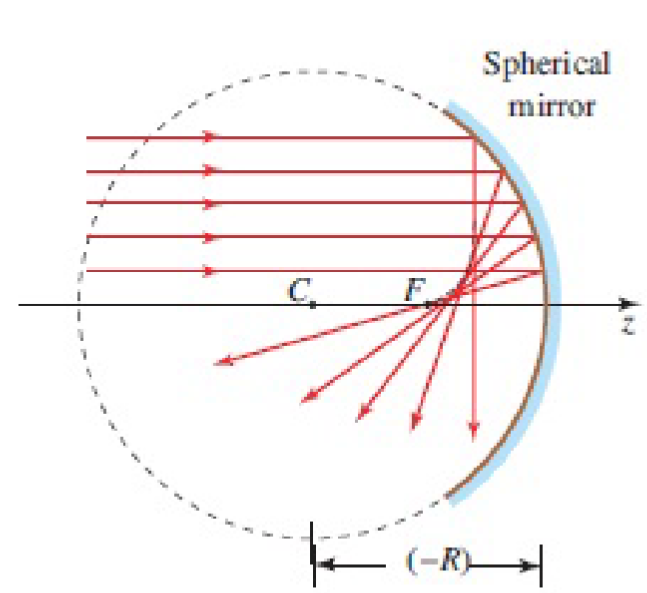
Mirror in the shape of a sphere
Different parallel rays focus on the axis at different points
Rays that are close enough to the axis will approximately focus at $\frac{R}{2}$ from the center
This is due to the small angle approximation ($\sin \theta \approx \theta$), and the rays are known as paraxial rays
Can be concave or convex
The radius of curvature, $R$, is negative for concave mirrors and positive for convex mirrors
More on paraxial rays
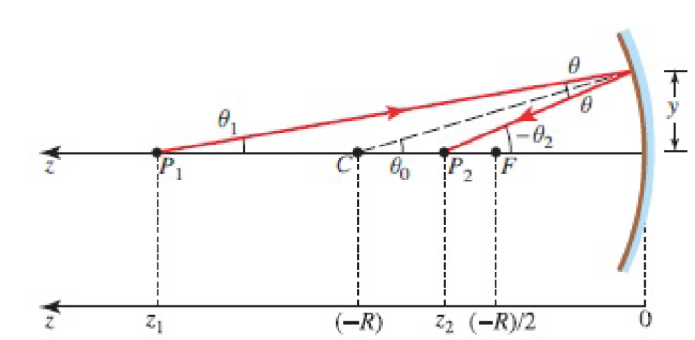
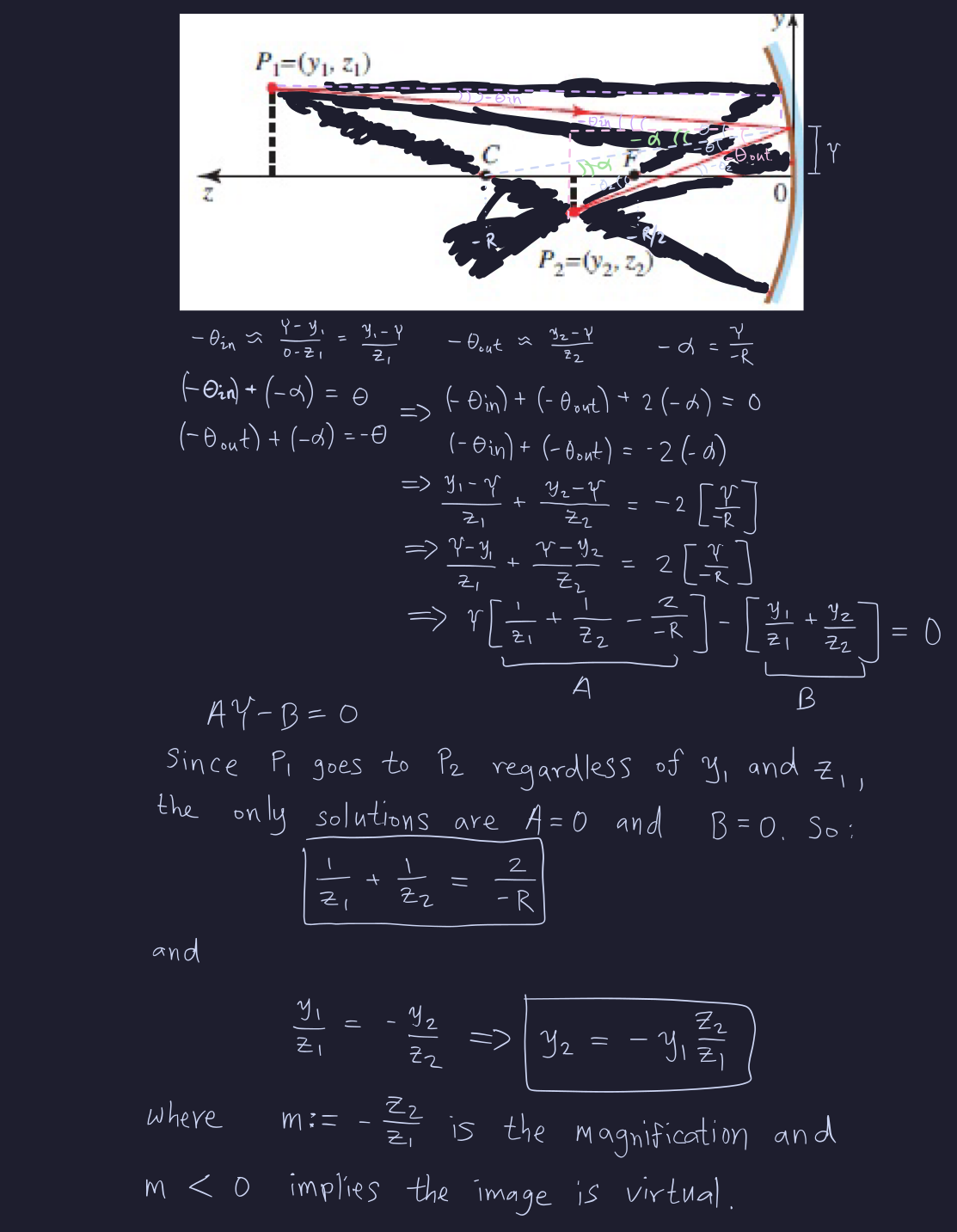
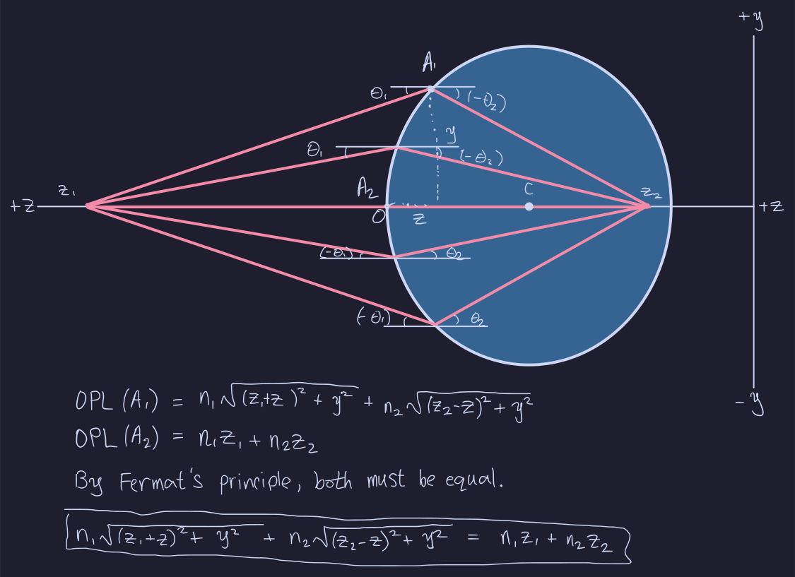
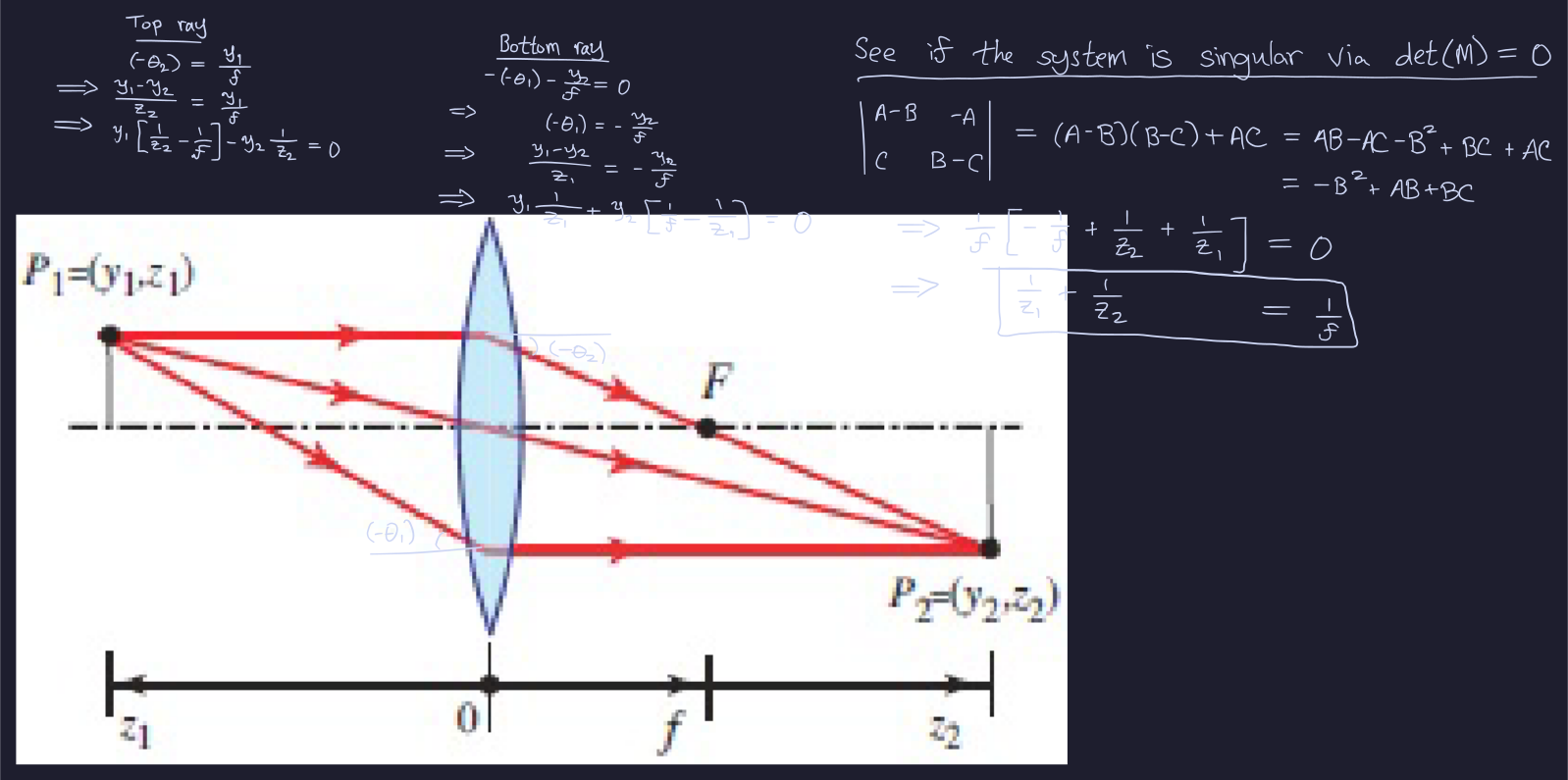
There is a one-to-one correspondence between paraxial rays originating from points on the mirror axis and their destination (image) points, which also lie on the mirror axis
Using angle relationships, we have $\theta_{1} = \theta_{0}-\theta \implies 2\theta_{0} = \theta_{1} + (-\theta_{2})$
If $\theta_0$ is small enough, $\tan \theta_{0} \approx \theta_{0}$, which gives $\frac{2y}{(-R)} \approx \theta_{1} + (-\theta_{2})$
And if $\theta_1$ and $(-\theta_2)$ are small enough, we have $\frac{2}{(-R)} \approx \frac{1}{z_{1}} + \frac{1}{z_{2}}$
If $z_1 = \infty$, then $z_2 = \frac{(-R)}{2} = f$. This results in the imaging equation for paraxial rays:
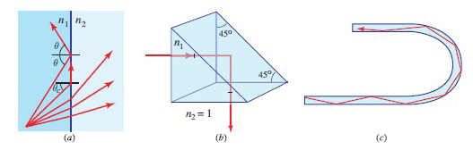
This is because $\theta_2$ is capped at $\frac{\pi}{2}$ rad, so beyond some critical $\theta_{c} \coloneqq \sin^{-1} \frac{n_{2}}{n_{1}}$, the planar boundary is treated like a normal reflecting surface
Prisms
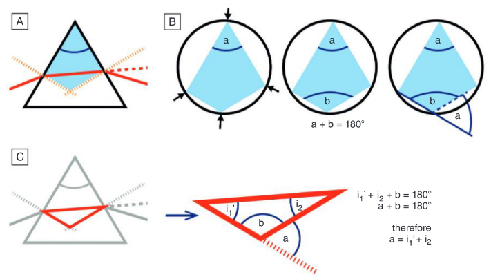
Characterization
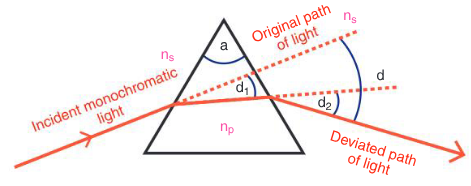
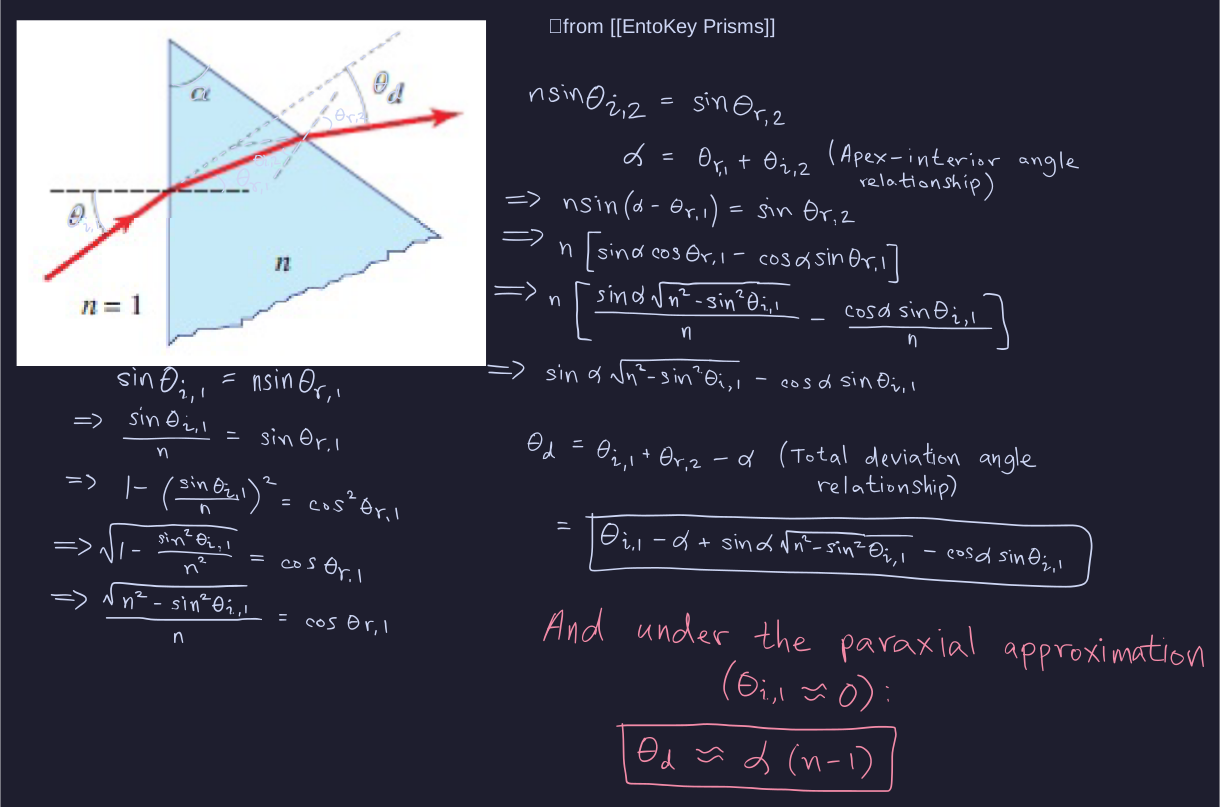
Characterized by the apical angle $\alpha$, refractive index $n$, and incident angle $\theta_{i,1}$
Derived values: first refracted ray $\theta_{r,1}$, first angle of deviation $\theta_{d,1}$, second incident ray $\theta_{i,2}$, second refracted ray $\theta_{r,2}$, second angle of deviation $\theta_{d,2}$, and total deviation $\theta_{d}$
Apex-interior relation (if you are solely working with first refracted/second incident rays—requires drawing normal lines): $\alpha = \theta_{r,1} + \theta_{i,2}$
Calculated using cyclic quadrilaterals[Course handout, Introduction to Visual Optics: A Light Approach, p. 102] (more on them here [Course handout, Cyclic Quadrilaterals])
Total deviation relation (easier imo—extend the path light takes, and calculate each deviation angle individually, then sum): $\theta_{d} = \theta_{d,1} + \theta_{d,2}$
Derivation[Saleh & Teich, Fundamentals of Photonics, p. 172]
Beamsplitters
Splits rays into a reflected and transmitted ray
Proportions of light split are determined by Fresnel's equations
Also used to combine two rays into one
Constructed via a thin metallic/dielectric film on a glass substrate
Beam Directors
Direct rays in arbitrary directions
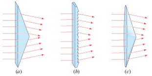
Biprism moves incident rays towards the central axis
Simplest biprism is a normal prism and inverted prism combined together into one isosceles triangle
Fresnel biprism is functionally identical to the simplest biprism but is formed from rows of adjacent, tiny prisms
Plano-convex axicon is a cone that collects incident rays in a circle and directs them towards the central axis (not just laterally like the first two; literally ALONG the central line)—shares the same cross section as simplest biprism (isosceles triangle)
Spherical Boundaries and Lenses
Spherical Boundaries
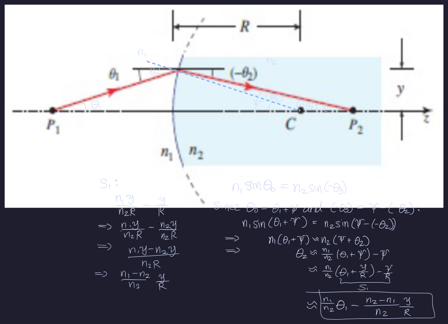
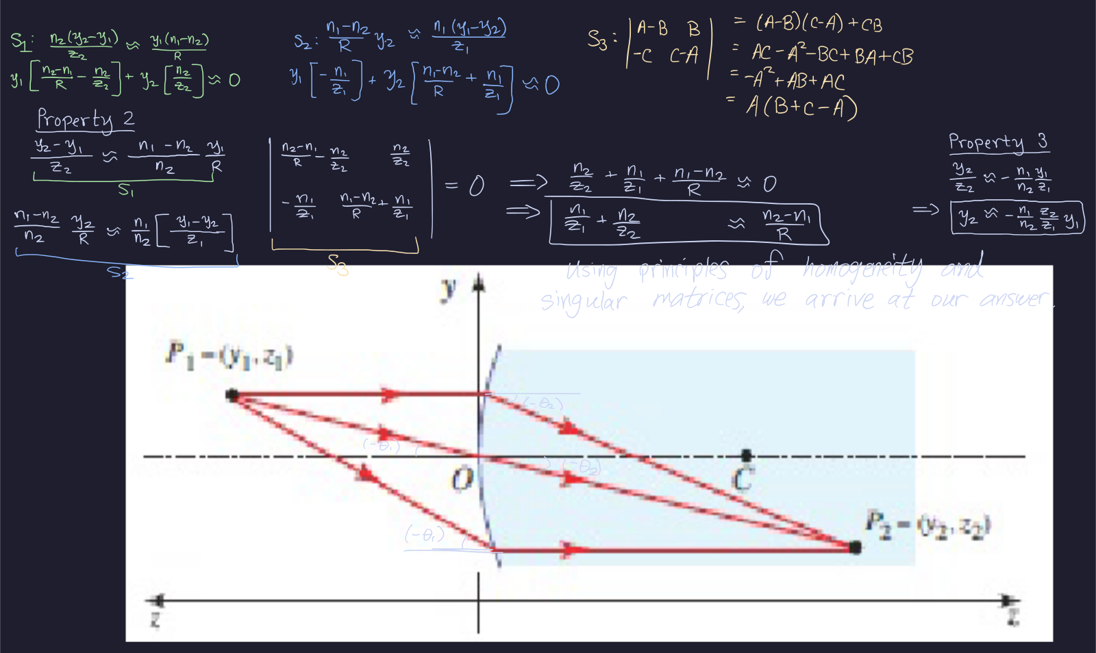
Consider a spherical boundary with radius $R$ between two media with refractive indices $n_1$ and $n_2$
Recall sign convention: $R > 0$ for convex; $R < 0$ for concave (obtained using Snell’s Law)
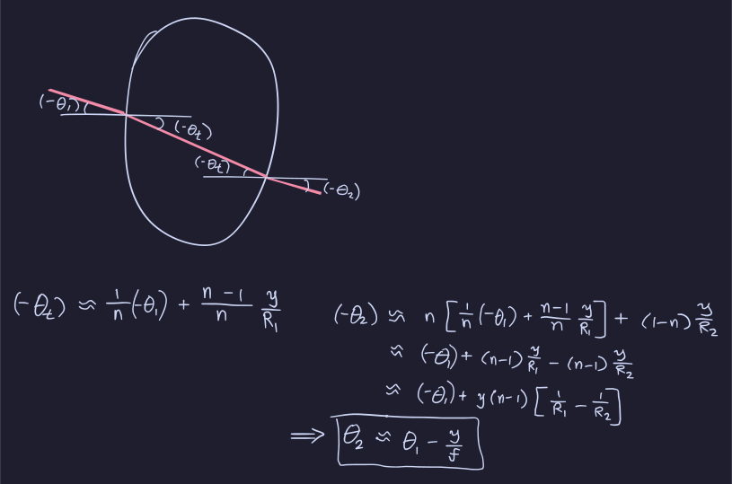
Measures how much the ray changes direction at the $z$-axis
and the resulting ray is extended until the second boundary
$\theta_2$ then becomes $\theta_1$ and the property is applied again for the exiting ray
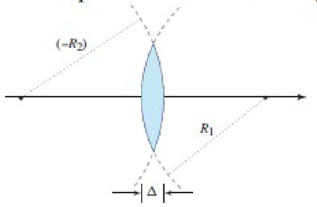
“Thin Lens” Assumption
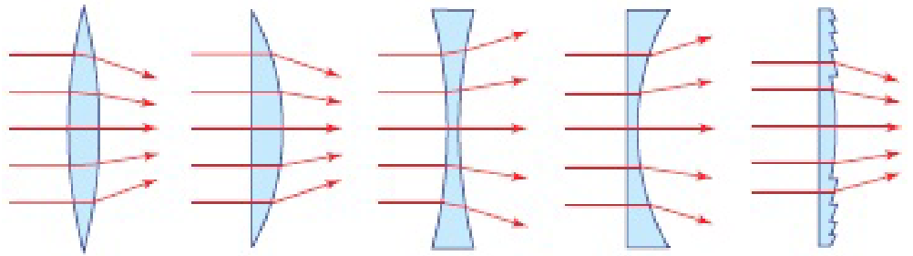
If the lens is thin, we may assume the emergent ray has approximately the same $y$ as the incident ray. In addition to simplifying things (we only have to track two angles, not four), this yields the following properties:
Often made with silica glass (a.k.a. fused silica/amorphous silicon dioxide ($\text{SiO}_{2}$)) due to its excellent optical/mechanical properties
Refractive index can be modified via doping (often with $\text{GeO}_{2}$)
TIR Reflection Condition
Definition(Notation peculiarities in this section).
My notation:
Overbar $\coloneqq$ measured from the surface normal
Unbarred $\coloneqq$ measured from the optical axis
Subscript $c$ marks the critical value of the variable it is attached to.
This reverses Saleh’s notation in the book (p. 185 [Saleh & Teich, Fundamentals of Photonics, p. 185]), where $\theta_c \coloneqq \sin^{-1}(n_2/n_1)$ and $\bar{\theta}_c \coloneqq 90^\circ - \theta_c$.
In other words: $\bar{\theta}_{c}$ here $=$ $\theta_{c}$ in the main TIR note. The unbarred $\theta_c$ here is fiber-specific and has no counterpart there.
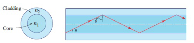
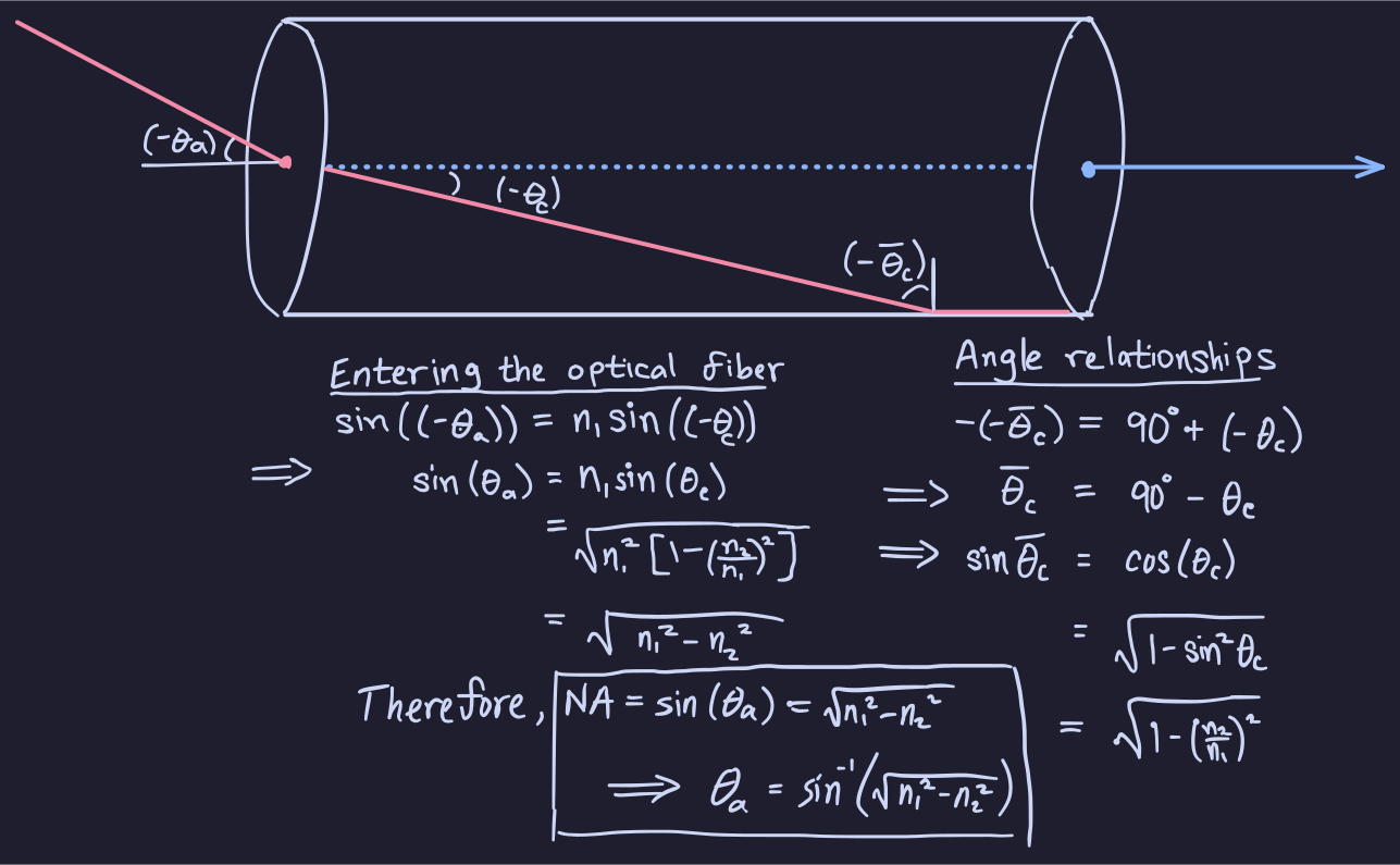
The cone of acceptable rays without undergoing refraction at the cladding is characterized by the half-angle, $\theta_a$, (a.k.a. the acceptance angle):
Proof of Cone of Acceptable Rays. (EXERCISE 1.2-5[Saleh & Teich, Fundamentals of Photonics, p. 187])
Light Trapping
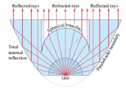
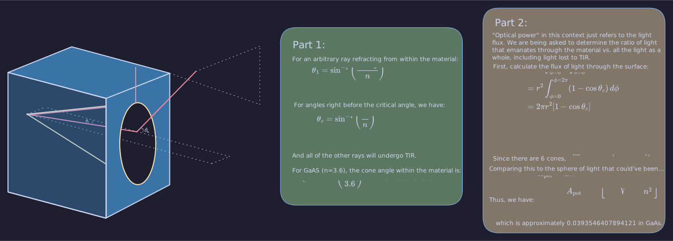
Light inside a medium with $n \gg 0$ can be “trapped” from entering air if the surfaces of the medium are parallel
The rays can undergo multiple TIRs without refracting into air
Exercise(Light Trapped in an LED).
(EXERCISE 1.2-6[Saleh & Teich, Fundamentals of Photonics, p. 189])
Graded-Index Optics
Graded-index (GRIN) materials have $n \equiv n(\bf{r})$
This causes curvature in light rays
Fabricated via impurities of controlled concentrations
Based on the $n(\bf{r})$, the GRIN can emulate a conventional optical component (prism/lens)
The Ray Equation
Main Equation
Theorem(Ray Equation).
Determines the trajectories of light rays in an inhomogeneous medium.
$$\frac{\mathrm{d}}{\mathrm{d}s} \left( n \frac{\mathrm{d}\mathbf{r}}{\mathrm{d}s} \right) = \nabla n $$
Proof of Ray Equation.
Assume the path is parametrized by $\bf{r}(s) \coloneqq \langle x(s), y(s), z(s) \rangle$. Using
Theorem(Euler-Lagrange Equation).
For a functional of the form
$$\int L(x, y, z, x^{'}, y^{'}, z^{'}) \ \mathrm{d}s,$$
the path that minimizes/maximizes the integral is determined by the following equations:
$$\frac{d}{ds}\left(\frac{\partial L}{\partial x'}\right) - \frac{\partial L}{\partial x} = 0 \quad \text{(and similarly for } y, z\text{)}.$$
on Fermat’s Principle, we account for the arc-length constraint $\left(\frac{dx}{ds}\right)^2 + \left(\frac{dy}{ds}\right)^2 + \left(\frac{dz}{ds}\right)^2 = 1$ via Lagrange multipliers. The augmented Lagrangian is:
For the actual ray trajectory, the Lagrange multiplier identifies with the refractive index: $\lambda(s) = \frac{n(\mathbf{r}(s))}{2}$. This yields three separate PDEs:
These three equations can be compactly written as the vector equation: $\frac{d}{ds}\left(n\frac{d\mathbf{r}}{ds}\right) = \nabla n$.
In general, the way you would solve the Ray Equation is by describing the trajectory by two functions and writing $\mathrm{d}s = \mathrm{d}z \sqrt{ 1 + \left( \frac{\mathrm{d}x}{\mathrm{d}z} \right)^2 + \left( \frac{\mathrm{d}y}{\mathrm{d}z} \right)^2 }$
Paraxial Regime
Corollary(Paraxial Ray Equations).
Under the paraxial approximation, the trajectory is nearly parallel to the $z$-axis, such that $\mathrm{d}s \approx \mathrm{d}z$. This simplifies the Ray Equation to:
$$\frac{\mathrm{d}}{\mathrm{d}z}\left( n \frac{\mathrm{d}x}{\mathrm{d}z} \right) \approx \frac{\partial n}{\partial x}, \ \ \ \frac{\mathrm{d}}{\mathrm{d}z}\left( n \frac{\mathrm{d}y}{\mathrm{d}z} \right) \approx \frac{\partial n}{\partial y}$$
which are much easier to solve for $x(z)$ and $y(z)$.
Graded-Index Optical Components
GRIN Slab
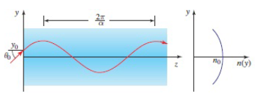
A slab of material with $n$ uniform in the $x$ and $z$ directions and varying in the $y$ direction
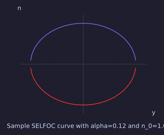
Special variant: SELFOC Slabs have a parabolic profile with $\alpha^2 y^2 \ll 1$
GRIN Fiber
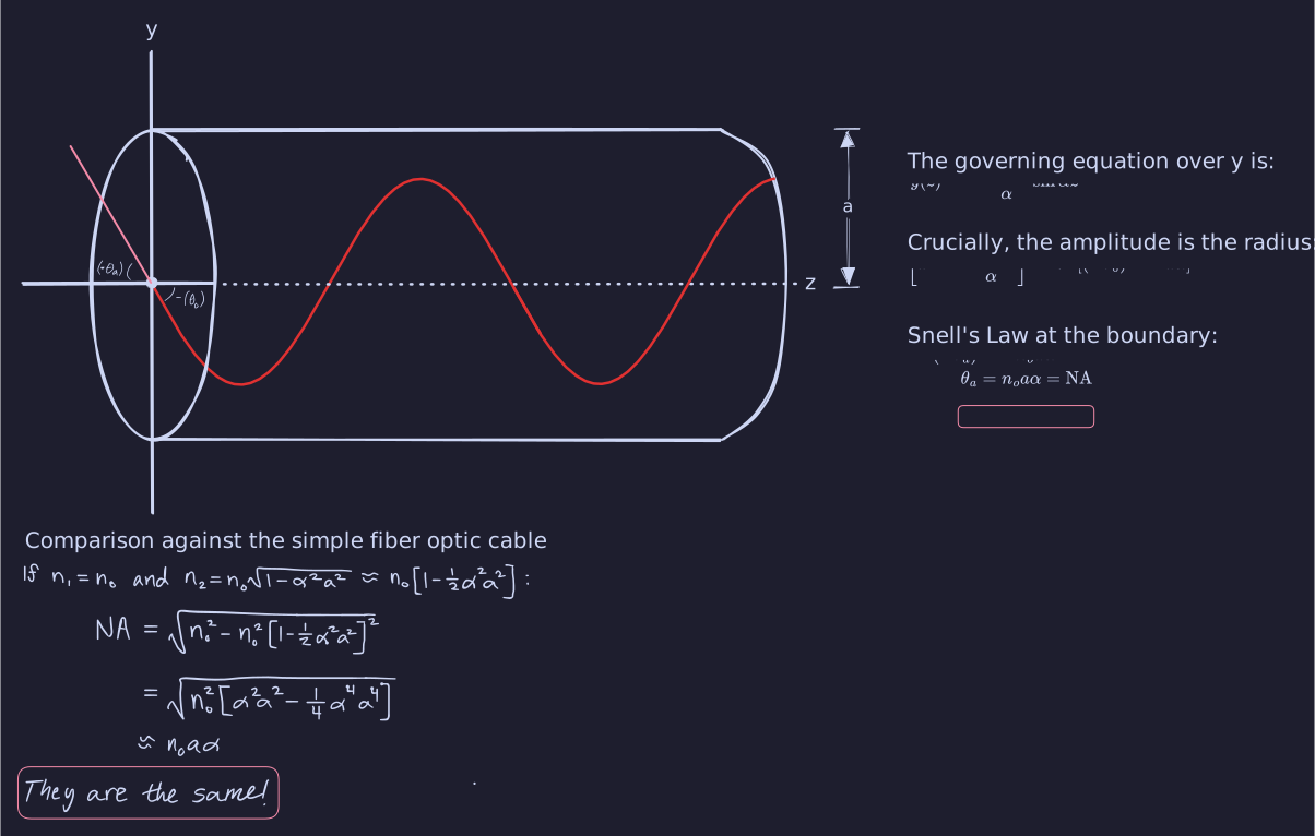
A glass cylinder with $n$ dependent on radial distance
Commonly used in optical fibers
Graded-Index Slab
Definition(GRIN Slab Relation).
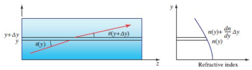
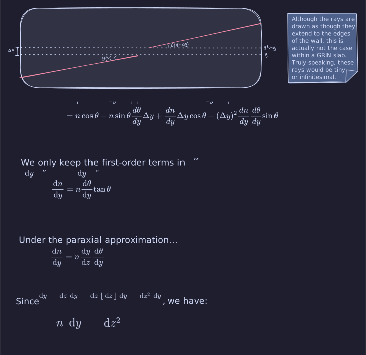
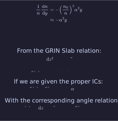
For a slab with $n=n(y)$, the rays in the $yz$-plane are described by:
$$\frac{\mathrm{d}}{\mathrm{d}z}\left( n \frac{\mathrm{dy}}{\mathrm{d}z} \right) = \frac{\mathrm{d}n}{\mathrm{d}y}, $$
Ray confinement: the rays stay confined to the SELFOC slab via TIR iff $2y_{\text{max}} < \text{slab thickness}$
One important condition for this analysis to hold:
$\theta_{\text{max}}$ is still paraxial: the max angle maintaining paraxiality implies that the ray trajectory approximation is indeed valid for all values of $z$ (i.e., $theta$ doesn’t grow unbounded)
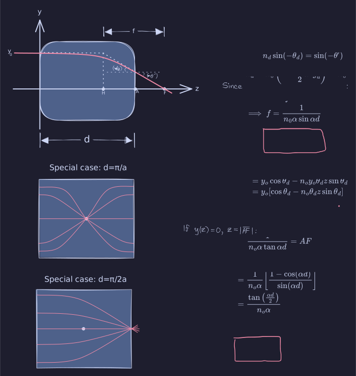
Exercise(The GRIN Slab as a Lens).
(EXERCISE 1.3-1[Saleh & Teich, Fundamentals of Photonics, p. 197])
Graded-Index Fibers
Definition(GRIN Fiber Relation).
Consider the sample distribution $n^2 = n_{0}^{2}\left[ 1-\alpha^2(x^2 + y^2) \right].$
Plugging it into the Ray Equation > Paraxial Ray Equations and assuming $\alpha_{2}(x+y_{2}) \ll 1$ for all $(x, y)$ of interest, we obtain:
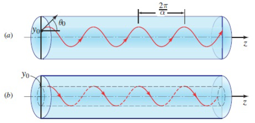
Thus, both $x(z), y(z)$ are harmonic with $T=\frac{2\pi}{\alpha}$.
The ICs $(x_0, y_0)$ and $(\theta_{x, 0}, \theta_{y, 0})$ determine the amplitude and phase.
If we let $x_0 = 0$ (valid because the solutions are axially symmetric), our solutions take the form:
$$\begin{align}
x(z) &= \frac{\theta_{x, 0}}{\alpha} \sin \alpha z \\
y(z) &= \frac{\theta_{y,0}}{\alpha} \sin \alpha z + y_{0} \cos \alpha z.
\end{align}$$
Two cases:
If $\theta_{x,0}=0$, the ray lines in a meridional plane through the cylinder axis; it follows a sinusoid like the Graded-Index Slab
If $\theta_{y,0}=0$ and $\theta_{x,0}=\alpha y_0$, then the ray becomes a helix that wraps a cylinder with radius $y_0$. In this case, $x(z) = y_0 \sin \alpha z$ and $y(z) = y_0 \cos \alpha z$.
Exercise(Numerical Aperture of the Graded-Index Fiber).
(EXERCISE 1.3-2[Saleh & Teich, Fundamentals of Photonics, p. 200])
The Eikonal Equation
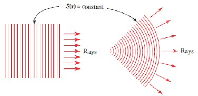
Ray trajectories are often characterized by the surface normal
The eikonal is a scalar function whose level surfaces define the direction of the ray trajectories via the normal
This follows from the fact that the normal to any level surface is always the gradient
For this reason, ray optics can be derived ab initio via Fermat’s Principle or the Eikonal Equation. By the Fundamental Theorem of Line Integrals, we have $S(\bf{r}_B)-S(\bf{r}_A)$ as the optical path length (line integral of $n$ from $A$ to $B$).
Matrix Optics
Matrix optics is a technique for ray tracing
Under this formalism, all rays are assumed to lie within a single plane and be paraxial
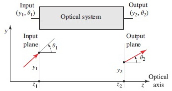
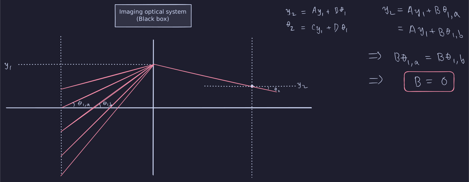
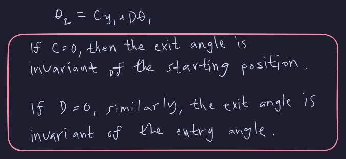
The positions and angles of the input and output planes are related by linear equations, which can then be encoded as a ray-transfer matrix
Highly convenient because the procedure generalizes for wider systems
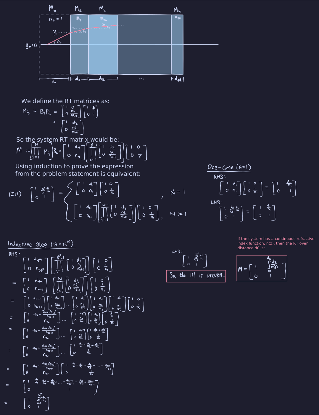
The RT matrix for a cascade of optical components/systems is a product of the RT matrices of the individual components
The RT Matrix
Consider a circularly symmetric system with many optical components centered around the $z$-axis
Rays in the $yz$-plane containing the optical axis cross two transverse planes at $z_1$ and $z_2$ are different axial distances
These rays are characterized by the $y$-coordinate of the crossing point and angle with the normal, $\theta$