Determining Frequency Response Experimentally

• A function generator conducts a “sweep” of frequencies as input to circuit
• Spectrum analysis is shown in oscilloscope output
  • Typically, a bode plot of gain and phase

Gain, Phase Shift, and Transfer Function

• We may express the input/output of any circuit variable (voltage, current, power) as phasors, measuring the amplitude and phase
• The frequency response is characterized by:
  • Gain $(A_x)$: ratio of output and input amplitudes
  • Phase shift $(\phi_x)$: difference between output and input phases
• Thus, we may define the Transfer function, $H(j \omega)$, as the ratio of the output and input phasors
  • Combines the above by characterizing the input-output relationship as a phasor (magnitude is gain and phase is phase shift)
  • May be used to determine the frequency response for sinusoidal inputs

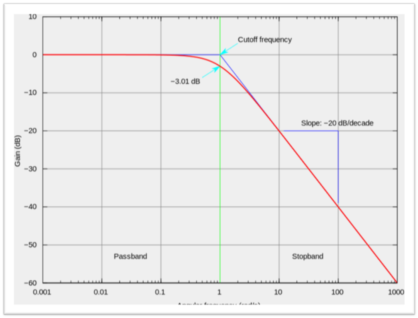
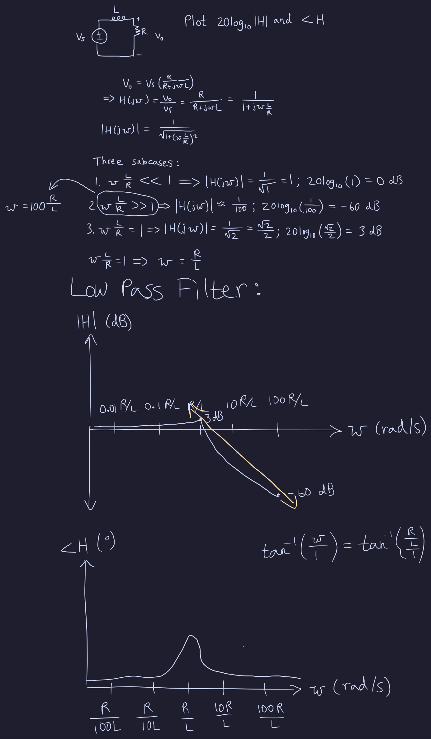
Bode Plot

• Two subplots:
  1. Measures $|H|$ vs $\omega$
  2. Measures $\angle H$ vs $\omega$
• Uses a $\log_{10}$ $x$-axis scale
• The slope of $|H|$ at $\omega >> 0$ determines how quickly the magnitude of the signal changes for every tenfold increase in frequency, in dB/decade
  • “Decade” here means tenfold increase, not an actual decade of time
  • This gives an asymptotic line that can help you better graph the plot

Example 07.1.

MATLAB

• Sample HPF code:

1R = 1e4;
2L = 10e-3;
3C = 100e-6;
4w = logspace(0, 5, 40);
5temp = (w * L - 1 ./ (w*C));
6gain = w*L ./ sqrt(R**2 + temp .^ 2);
7phi = -atand(temp / R);
8figure(1), semilogx(w, gain), grid;
9figure(2), semilog(w, phi), grid;

RLC Filters

• RLC circuits effectively act as bandpass filters since they have two energy storage components (L and C).
• At the resonant frequency $\omega_0 = \frac{1}{\sqrt{LC}}$, the gain is maximized (typically normalized to unity in passive systems).

Drop-off Frequencies

• Defined as the frequencies where the gain drops to -3 dB from the peak (i.e., $\frac{1}{\sqrt{2}}$ of max).
• For a standard series RLC:
  • High drop-off frequency: $\omega_{\text{high}} = \omega_0 + \frac{R}{2L}$
  • Low drop-off frequency: $\omega_{\text{low}} = \omega_0 - \frac{R}{2L}$
  • Approximate bandwidth: $\Delta \omega = \omega_{\text{high}} - \omega_{\text{low}} = \frac{R}{L}$
• In terms of simpler low/high-frequency approximations:
  • High drop-off: $\frac{R}{L}$
  • Low drop-off: $\frac{1}{RC}$

Cutoff Frequencies

• Defined here as the frequencies where gain drops to -20 dB (i.e., 10 times further from the peak than -3 dB).
• Rule-of-thumb estimations:
  • High cutoff: $\omega_{\text{cutoff, high}} = 10 \cdot \frac{R}{L}$
  • Low cutoff: $\omega_{\text{cutoff, low}} = \frac{1}{10RC}$

Generalized Second-Order Circuits with Complex Roots

• Only applicable to underdamped systems where the characteristic equation has complex roots
• The general form of the transfer function is:

where $\zeta = \frac{\alpha}{\omega_{0}}$

• Behavior depends on how $\omega$ compares to the natural frequency $\omega_0$:

Three Subcases:

1. Low-frequency regime: $\omega \ll \omega_0$
   • Magnitude: $|H| \approx k$
   • Phase: $\angle H \approx 0^\circ$
2. At resonance: $\omega = \omega_0$
   • Magnitude: $|H| = \frac{k}{2\zeta}$
   • Phase: $\angle H = -90^\circ$
3. High-frequency regime: $\omega \gg \omega_0$
   • Dominant term is $-\left( \frac{\omega}{\omega_0} \right)^2$ in the denominator
   • Magnitude: $|H| \approx \frac{k \omega_0^2}{\omega^2}$ (i.e., rolls off as $1/\omega^2$)
   • Phase: $\angle H \approx -180^\circ$

General Second-Order Transfer Function Decomposition

• All second-order circuits can be written as a transfer function in “standard form”:
  • If it is not already in this form, you must perform partial fraction decomposition

• This overall transfer function may be broken down as the product of three simpler transfer functions:

where

• $H_1 = k$

• $H_2 = \frac{1}{1 + j \omega / p_1}$

• $H_3 = \frac{1}{1 + j \omega / p_2}$

• Each of these simpler transfer functions corresponds to a first-order low-pass filter or a gain term

• $p_1$ and $p_2$ are the pole frequencies of the system (complex conjugates in the underdamped case, real in overdamped)

• The expression $1 + j \omega / p_i$ is not the pole itself, but a standard form for expressing frequency-domain behavior near that pole

Log-Magnitude Decomposition

• The overall magnitude in decibels is the sum of the magnitudes:

References

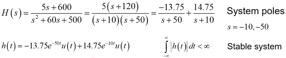
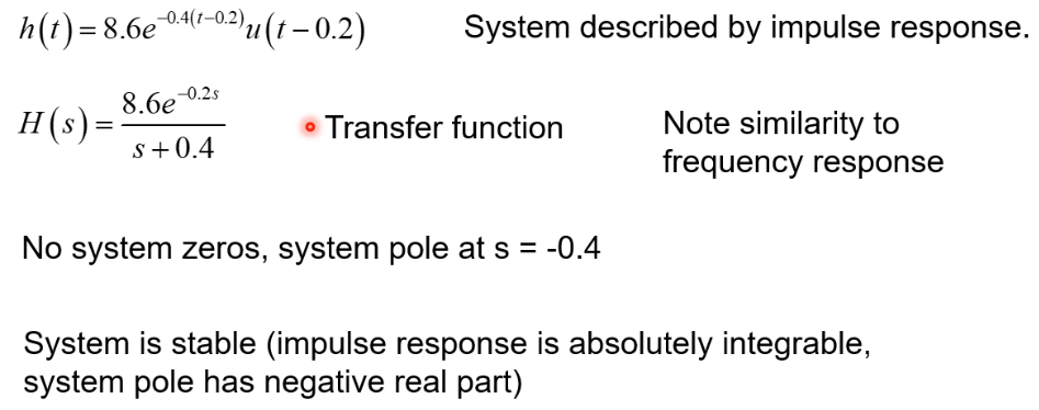
• Transfer (System) Functions

  • The ratio of the Laplace transform of the system output to the Laplace transform of the system input

  $$H(s) = \frac{Y(s)}{X(s)}$$

  • Can also be determined by taking the Laplace transform of the impulse response or from differential equations describing the system

  $$H(s) = \int_{-\infty}^{\infty}h(t)e^{-st} \ \mathrm{d}t$$

  Poles and Zeros

  • Roots of $Y(s)$ are the system zeros
  • Roots of $X(s)$ are the system poles ($\mathcal{P}$)

  $$\forall p \in \mathcal{P}, \Re(p) < 0 \implies \int_{-\infty}^{\infty} |h(t)| \, dt < \infty \implies \text{BIBO stability}$$

  

  References

  • Transfer functions (course handout)

• Continuous-time Systems

  • Represented by:
    • Differential equation
    • Impulse response (convolution integral)
    • Frequency response
    • Transfer function
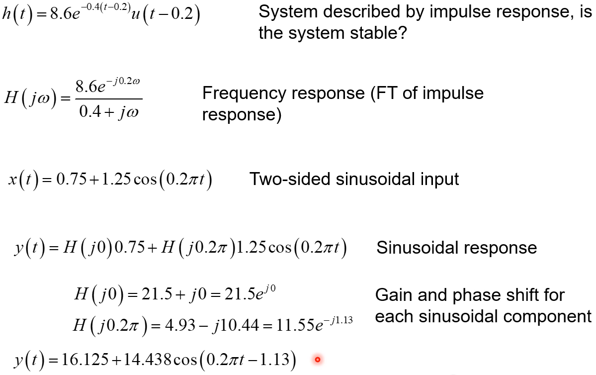
  • Impulse response, $h(t)$, is the system response to $\delta$
  • LTI system is BIBO stable if its impulse response is absolutely integrable

  $$ h(t) = y(t) \ \vert_{x(t) = \delta(t)} $$$$ y(t) = h(t) * x(t) = \int_{-\infty}^{\infty} = h(\tau)x(t-\tau) \ \mathrm{d}\tau $$

  Frequency Response

  • Describes what the system does to sinusoidal inputs
  • Broken down into magnitude and phase components

  $$H(j\omega) = \vert H(j\omega) \vert \angle H(j\omega)$$

  • Determined using the Fourier transform of $h(t)$

  $$H(j\omega) = \int_{-\infty}^{\infty}h(t)e^{-j\omega t} \ \mathrm{d}t$$

  Analysis of $H(j\omega)$

  Let $H(j\omega)$ be a general frequency response function of the form $H(jω)= \frac{N(j\omega)}{D(j\omega)}$. Then:

  • $|H(j\omega)| = \frac{|N(j\omega)|}{|D(j\omega)|}$
  • $H(j\omega) = \angle N(j\omega) - \angle D(j\omega)$

  Magnitude Calculation

  • If $M(j\omega) = A e^{j\phi(\omega)}$, $|M(j\omega)| = A$
  • If $M(j\omega) = a + j b(\omega)$, $|M(j\omega)| = \sqrt{a^2 + b(\omega)^2}$

  Phase Calculation

  • If $M(j\omega) = A e^{j\phi(\omega)}$, $\angle M(j\omega) = \phi(\omega)$
  • If $M(j\omega) = a + j b(\omega)$, $\angle M(j\omega) = \tan^{-1}\left(\frac{b(\omega)}{a}\right)$

  Sinusoidal Response

  • Response to sinusoids for an LTI system is a sinusoid of the same frequency with a shifted amplitude (gain) and phase, dependent on $H(j\omega)$
  • Frequencies of the sinusoidal components cannot change and it must be two-sided
  • Input format $x(t)$:

  $$x(t) = A_{0} + \sum_{k=1}^{N}A_{k}\cos(\omega_{k}t + \phi_{k})$$

  • Output format $y(t)$:

  $$y(t) = \vert H(j0) \vert A_{0} + \sum_{k=1}^{N} \vert H(j\omega_{k}) \vert A_{k} \cos(\omega_{k}t + \phi_{k} + \angle H(j\omega_{k}))$$

  

  References

  • Frequency response (course handout)

• Frequency Response and Filters 1 (course handout)

• Construction of Bode Diagrams

• Drawing Bode Diagrams