Notes › EENG 3345: AC Circuit Analysis Lecture 8
Laplace Transform
634 words 5 min Modified
Table of Contents
Laplace Transform
- Transforms differential equations into algebraic systems
- Solve the system and convert back to time domain
- LT of a signal $x(t)$:
$$ X(s) = \int_{-\infty}^{\infty} x(t) e^{-st} \, dt $$ - iLT of $X(s)$:
$$ x(t) = \frac{1}{j 2 \pi} \int_{c - j\infty}^{c + j\infty} X(s) e^{st} \, ds $$ - Use the table of pairs and properties [Laplace transform table (course handout)] to evaluate LT and iLT
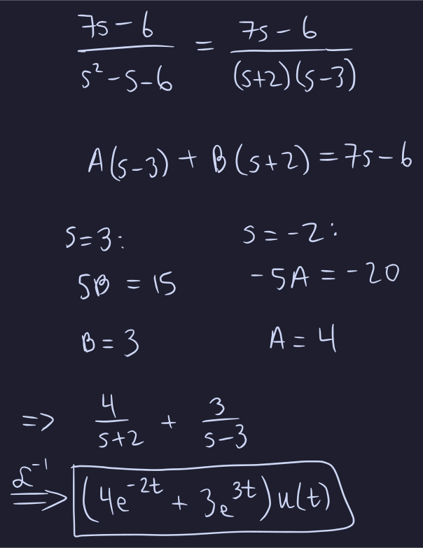
Example 08.1 (Find iLT of $\frac{7s - 6}{s^2 - s - 6}$).
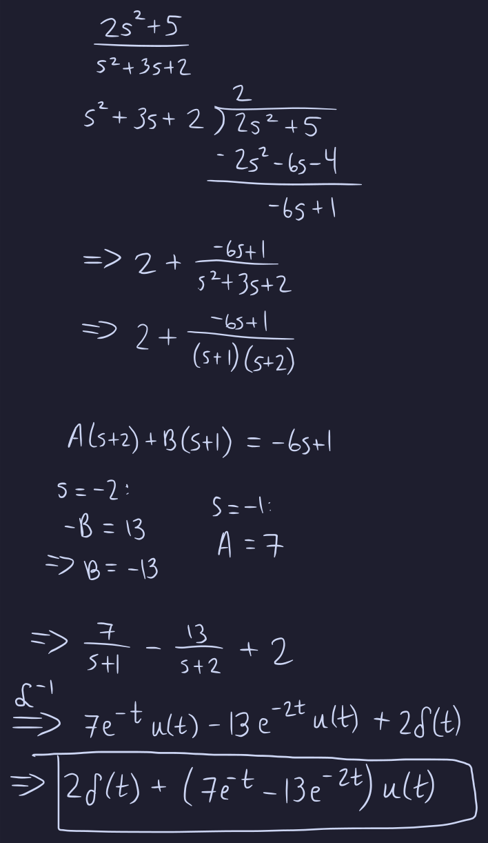
Example 08.2 (Find iLT of $\frac{2s^2 + 5}{s^2 + 3s + 2}$).
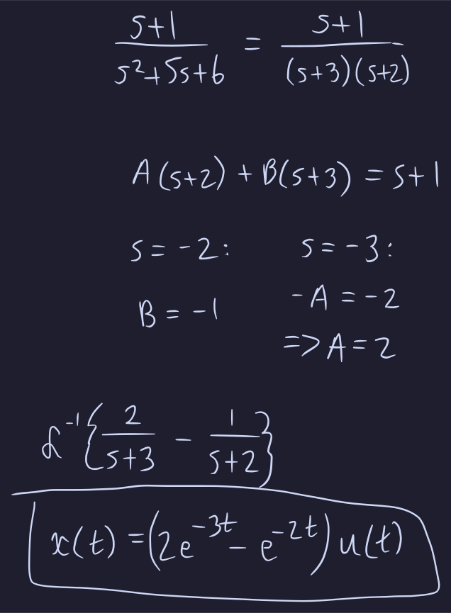
Example 08.3 (Find iLT of $\frac{s+1}{s^2 + 5s + 6}$).
Solving Circuits Using Laplace Transform
Transfer Function and System Response
- Take the Laplace transform of the system’s equations including any nonzero initial conditions and solve for $Y(s)$
- The $s$-domain output is:
$$ Y(s) = H(s) X(s) + Y_{\text{IC}}(s) $$ - where:
- $H(s)$ is the transfer function
- $X(s)$ is the Laplace transform of the input signal
- $Y_{\text{IC}}(s)$ is the Laplace terms resulting from the initial conditions
- This is obtained by setting $X(s) = 0$
- Take the inverse Laplace transform to get the time-domain output:
$$ y(t) = \mathcal{L}^{-1} \left\{ H(s) X(s) + Y_{\text{IC}}(s) \right\} $$ - This gives the total response as the sum of:
- Zero-state response: $$ y_{\text{ZS}}(t) = \mathcal{L}^{-1} \left\{ H(s) X(s) \right\} $$
- Zero-input response: $$ y_{\text{ZI}}(t) = \mathcal{L}^{-1} \left\{ Y_{\text{IC}}(s) \right\} $$
- So the complete output is: $$ y(t) = y_{\text{ZS}}(t) + y_{\text{ZI}}(t) $$
Domain Transformation
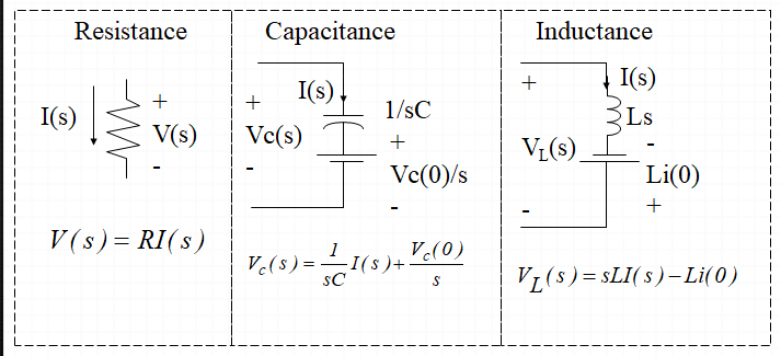
- Transform the circuit into the $s$-domain equivalent circuit:
- Resistors remain unchanged
- Inductors and capacitors may be modeled as $s$-impedances in series with an ideal independent voltage source
- Capacitor:
- Inductor:
- Solve for variables in the $s$-domain using methods of circuit analysis
- Apply inverse Laplace transform for time domain solution
(Special Case of Above) Sinusoidal Steady-State Analysis
- Assume all sources are sinusoidal and operating at the same frequency
- Transform the circuit into the phasor (frequency) domain
- Replace $s$ with $j\omega$ to convert from Laplace to steady-state analysis
- Replace elements with their steady-state impedances
- Resistor: $R$
- Inductor: $j\omega L$
- Capacitor: $\frac{1}{j\omega C}$
- Use phasor circuit analysis to solve for voltages and currents
- Convert phasor results back to time domain using
$$ x(t) = \Re \left\{ \tilde{X} e^{j\omega t} \right\} $$ where $\tilde{X}$ is the phasor representation of the signal
Initial and Final Value Theorem
- Useful so that you don’t have to solve for initial and final conditions of current/voltage using transient analysis
- Using IVT/FVT, we may rewrite the complete response of a first-order circuit as:
Initial Value Theorem (IVT)
$$ \lim_{t \to 0^+} f(t) = \lim_{s \to \infty} s F(s) $$Requirements:
- $f(t) \in \mathcal{L}\{f(t)\}$
- $\lim_{t \to 0^+} f(t) \in \mathbb{R}$
- $f(t) \not\ni \delta(t)$
Final Value Theorem (FVT)
$$ \lim_{t \to \infty} f(t) = \lim_{s \to 0} s F(s) $$Requirements:
- $f(t) \in \mathcal{L}\{f(t)\}$
- $\lim_{t \to \infty} f(t) \in \mathbb{R}$
- Let $\mathcal{P}$ be the set of poles of $s F(s)$. Then:
- $s = 0 \in \mathcal{P} \Rightarrow \operatorname{ord}_{s=0}(sF(s)) \le 1$
References
-
Continuous-Time Systems Analysis Laplace Transform 1 (course handout)
-
Laplace transform (course handout)
-
System Response Using Laplace Transform
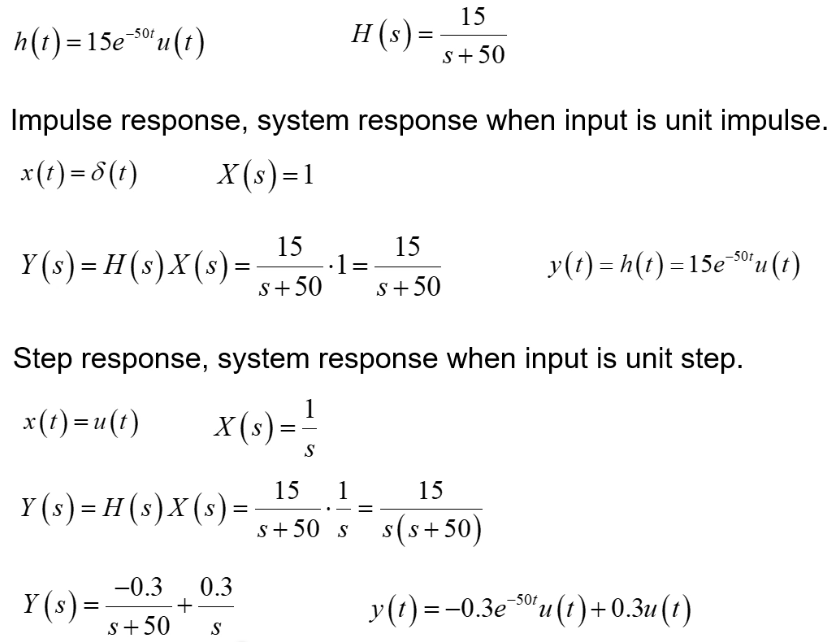
- Similar to Fourier System Response, multiplication in the $s$-domain is convolution in the time domain
- Take the product of the transfer function and the input in the $s$-domain, then take the inverse laplace transform
Using LTI Properties
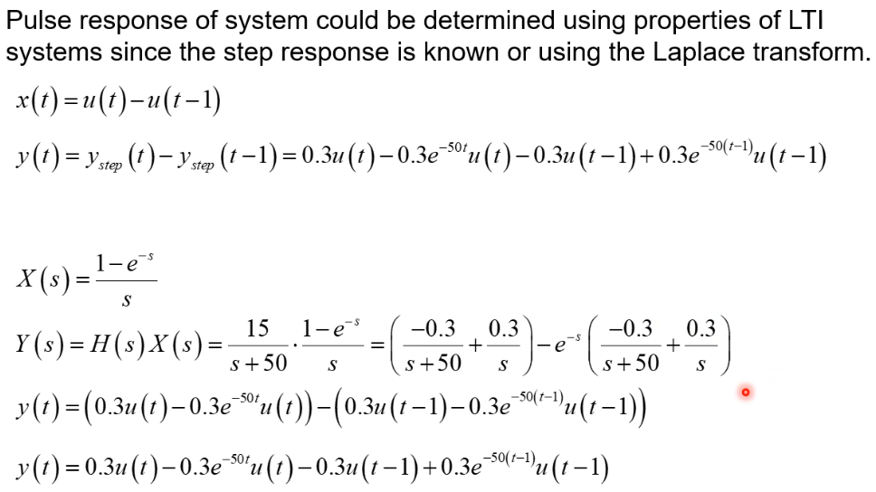
- May leverage linearity property of LTI systems if the step/impulse response is already known
Using MATLAB
-
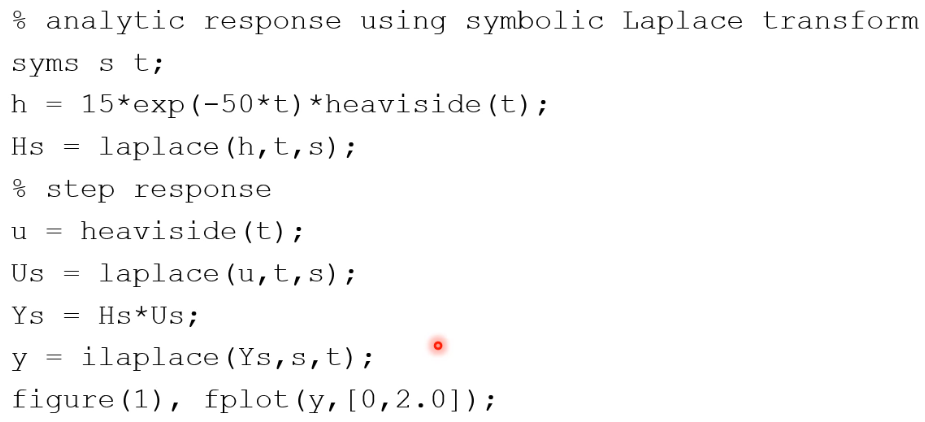
Analytic response with symbolic toolbox
-
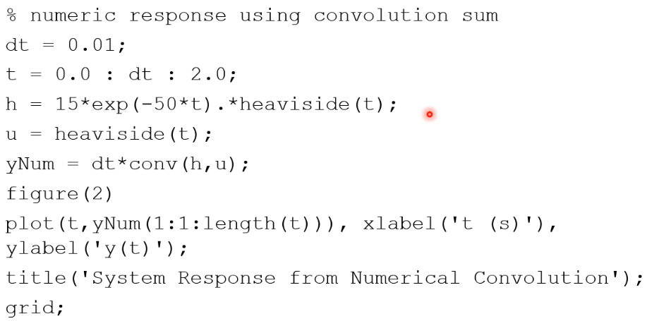
Numeric response (convolution sum)
-
Numeric response using built-in functions (
impulse,step,lsim)- Easiest method possible
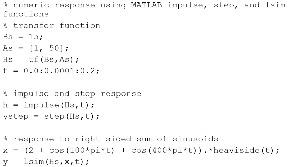
- Easiest method possible
References
- System response (course handout)
Sources
- Continuous-Time Systems Analysis Laplace Transform 1
- Laplace transform
- Laplace transform table (course handout)
- System response