Notes › EENG 3345: AC Circuit Analysis Lecture 9
Fourier Transform
322 words 2 min Modified
Table of Contents
Introduction
- FT decomposes a signal into its frequency components
- Unlike the Laplace Transform (which uses $s = \sigma + j\omega$), FT is restricted to $s = j\omega$
Continuous-Time Fourier Transform
- FT:
- iFT:
- Use the table of pairs and properties [Fourier transform table (course handout)] to evaluate FT/iFT
Solving Circuits Using Fourier Transform
- Although possible in some cases, it’s not really practical to use FT when dealing with initial conditions or systems involving transient behavior
- General rule of thumb: LT for response, FT for spectral analysis (which isn’t really covered in this course)
Transfer Function and System Response
- Use when the impulse response $h(t)$ and input $x(t)$ are both known
- Transform both signals:
- $H(j\omega) = \mathcal{F}\{ h(t) \}$
- $X(j\omega) = \mathcal{F}\{ x(t) \}$
- Multiply in frequency domain: $$ Y(j\omega) = H(j\omega) X(j\omega) $$
- Inverse transform to get output: $$ y(t) = \mathcal{F}^{-1} \left\{ Y(j\omega) \right\} $$
Domain Transformation
- Replace each circuit element with its Fourier-domain impedance
- Resistor: $R$
- Inductor: $j\omega L$
- Capacitor: $\frac{1}{j\omega C}$
- Take the FT of the input signal
- Solve the circuit using methods of circuit analysis
- Compute output in the Fourier domain
$$ Y(j\omega) = H(j\omega) X(j\omega) $$ - Take the iFT to find $y(t)$
$$ y(t) = \mathcal{F}^{-1} \left\{ Y(j\omega) \right\} $$
References
-
Fourier Transforms (course handout)
-
Fourier transform (course handout)
-
Using Fourier Transform
- It is possible to obtain the response of a continuous LTI system via Fourier transform
- Should only be used when:
- Convolution integral is not manageable
- Step responses are unknown (cannot leverage homogeneity/additivity)
- System is not a sum of sinusoids
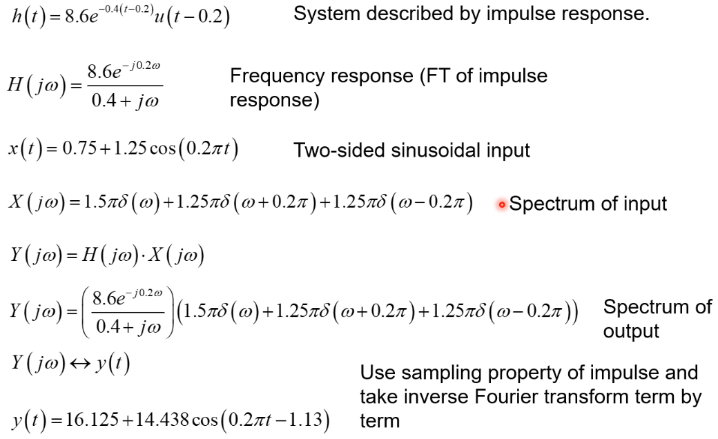
- For a system described by impulse response $h(t)$ and input $x(t)$:
- $x(t) \xrightarrow{\mathscr{F}}X(j\omega)$
- $h(t) \xrightarrow{\mathscr{F}}H(j\omega)$
- $X(j\omega) \cdot H(j\omega) = Y(j\omega)$
- $Y(j\omega) \xrightarrow{\mathscr{F}^{-1}}y(t)$
- This is possible due to convolution property of Fourier transform
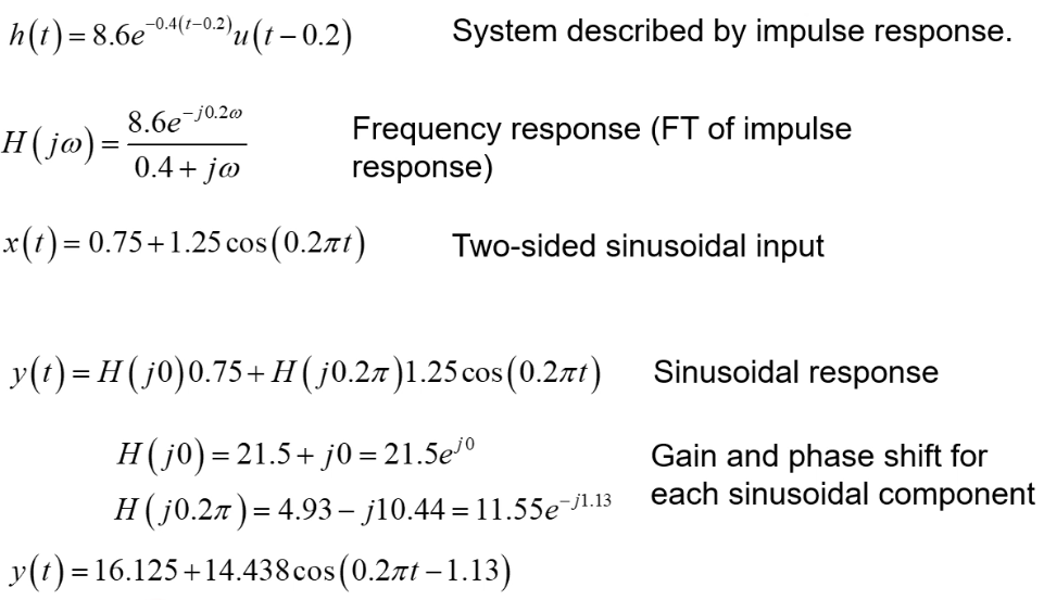
Using Sum of Sinusoids
References
- System response (course handout)
Sources
- Fourier Transforms
- Fourier transform
- Fourier transform table (course handout)
- System response