The Beauty of Spherical Harmonics, Part 3: Diagonalize and Decouple
Why does a drum have no clear pitch?
3401 words 25 min Modified
Table of Contents
Part 3 of 3 in The Beauty of Spherical Harmonics
- Building the Basis
- Solving Laplace's Equation
- Diagonalize and Decouple
Last time, we decomposed $V$ into $Y_{\ell m}$’s, watched the decomposition solve Laplace mode by mode, and got a feel for what $\ell$ and $m$ actually look like. That finishes the toolkit, so from here on it’s applications.
Truncation
Previously, we had
$$ f(\theta,\psi)=\sum_{\ell=0}^{\infty}\sum_{m=-\ell}^{\ell}c_{\ell m}Y_{\ell m}(\theta,\psi) $$What happens when the sum has to stop? A computer only holds finitely many $c_{\ell m}$. Pick a largest $\ell$, call it $\ell_{\max}$, and keep every shell up to it:
$$ f_{\ell_{\max}}(\theta,\psi)=\sum_{\ell=0}^{\ell_{\max}}\sum_{m=-\ell}^{\ell}c_{\ell m}Y_{\ell m}(\theta,\psi) $$As an operator, truncation is a sum of shell projectors:
$$ \begin{align*} \hat{P}_{\ell}&=\sum_{m=-\ell}^{\ell}\ket{\ell m}\bra{\ell m}\\ \hat{T}_{\ell_{\max}}&=\sum_{\ell=0}^{\ell_{\max}}\hat{P}_{\ell}\\ \ket{f_{\ell_{\max}}}&=\hat{T}_{\ell_{\max}}\ket{f} \end{align*} $$Cost: shell $\ell$ holds $2\ell+1$ coefficients, so
$$ \begin{align*} \sum_{\ell=0}^{\ell_{\max}}(2\ell+1)&=2\cdot\frac{\ell_{\max}(\ell_{\max}+1)}{2}\\ &\quad+(\ell_{\max}+1)\\ &=(\ell_{\max}+1)^2 \end{align*} $$What $\ell_{\max}$ Resolves
Previously, we had $\left< Y_{\ell m} \right>_{\varepsilon}-Y_{\ell m}\approx-\frac{\varepsilon^2}{4}\ell(\ell+1)Y_{\ell m}$. How wiggly is that, as a length? Zoomed in far enough, the sphere is flat, so compare a plane wave $\cos kx$ averaged over a ring of radius $s$:
$$ \begin{align*} \left<\cos kx\right>_{s}&=\frac{1}{2\pi}\int_{0}^{2\pi}\cos\left(kx+ks\cos\psi'\right)\mathrm{d}\psi'\\ &\approx\frac{1}{2\pi}\int_{0}^{2\pi}\Big[\cos kx-ks\cos\psi'\,\sin kx\\ &\qquad-\frac{k^2s^2}{2}\cos^2\psi'\,\cos kx\Big]\mathrm{d}\psi'\\ &=\left(1-\frac{k^2s^2}{4}\right)\cos kx \end{align*} $$$\cos\psi'$ integrates to $0$ and $\cos^2\psi'$ to $\pi$.
On a sphere of radius $R$, a ring of geodesic angle $\varepsilon$ has $s=R\varepsilon$. Matching the two:
$$ \begin{align*} \frac{k^2(R\varepsilon)^2}{4}&=\frac{\ell(\ell+1)\,\varepsilon^2}{4}\\ \implies kR&=\sqrt{\ell(\ell+1)}\\ &=\sqrt{\left(\ell+\tfrac{1}{2}\right)^2-\tfrac{1}{4}}\\ &\approx\ell+\tfrac{1}{2} \end{align*} $$Locally, $Y_{\ell m}$ is a wave that fits $\ell+\frac{1}{2}$ wavelengths around a great circle.
The finest bump a wave can draw is half a wavelength. So the finest bump $f_{\ell_{\max}}$ can draw, as an angle:
$$ \begin{align*} \Delta\theta_{\min}&\approx\frac{1}{2}\cdot\frac{2\pi}{\ell_{\max}+\frac{1}{2}}\\ &\approx\frac{\pi}{\ell_{\max}} \end{align*} $$So what is a good $\ell_{\max}$? Invert it. To resolve features of angular size $\Delta\theta$:
$$ \ell_{\max}\approx\frac{\pi}{\Delta\theta} $$$\Delta\theta=1^{\circ}=\frac{\pi}{180}$: $\ell_{\max}\approx180$, i.e. $181^2\approx3.3\times10^{4}$ coefficients. Earth’s gravity field (EGM2008) goes to $\ell_{\max}\approx2160$: $\frac{\pi R_{\oplus}}{2160}\approx9\text{ km}$ at the surface. Planck’s maps of the cosmic microwave background go to $\ell\approx2500$: features down to $\frac{\pi}{2500}\text{ rad}\approx4'$. Same rule from the data side: samples spaced by $\Delta\theta$ can’t pin down anything above $\ell_{\max}\approx\frac{\pi}{\Delta\theta}$ (two samples per wavelength).
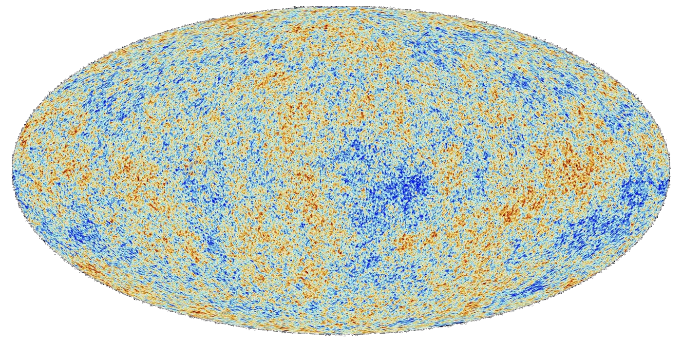

That’s resolution. How close is $f_{\ell_{\max}}$ to $f$? Previously, $\braket{\ell' m'}{\ell m}=\delta_{\ell\ell'}\delta_{mm'}$, so the error is just the coefficients that got dropped:
$$ \begin{align*} \left\|f-f_{\ell_{\max}}\right\|^2&=\braket{f-f_{\ell_{\max}}}{f-f_{\ell_{\max}}}\\ &=\sum_{\ell,\ell'>\ell_{\max}}\;\sum_{m,m'}c_{\ell' m'}^*\,c_{\ell m}\braket{\ell' m'}{\ell m}\\ &=\sum_{\ell>\ell_{\max}}\underbrace{\sum_{m=-\ell}^{\ell}|c_{\ell m}|^2}_{E_{\ell}} \end{align*} $$$E_{\ell}$ is shell $\ell$’s share of $\|f\|^2$. How fast it dies depends only on how smooth $f$ is.
Finite sum: exact at a finite $\ell_{\max}$. Previously,
$$ V_0\cos^2\theta=\frac{V_0}{3}P_0(\cos\theta)+\frac{2V_0}{3}P_2(\cos\theta) $$so $\ell_{\max}=2$ is exact.
Smooth bump of angular width $\sigma$ (at the pole, so only $m=0$). In flat space, a Gaussian of width $R\sigma$ has Fourier transform $\propto e^{-k^2(R\sigma)^2/2}$, and $k^2R^2=\ell(\ell+1)$ from above:
$$ c_{\ell 0}\propto\sqrt{2\ell+1}\;e^{-\ell(\ell+1)\sigma^2/2} $$The $\sqrt{2\ell+1}$ is from $N_{\ell 0}$ and grows too slowly to matter. Demand that the last kept coefficient is down by a factor $\delta$:
$$ \begin{align*} e^{-\ell_{\max}(\ell_{\max}+1)\sigma^2/2}&=\delta\\ \implies\ell_{\max}&\approx\frac{\sqrt{2\ln(1/\delta)}}{\sigma} \end{align*} $$$\delta=10^{-3}$ gives $\ell_{\max}\approx\frac{3.7}{\sigma}$, the same size as $\frac{\pi}{\sigma}$. Checked numerically at $\sigma=0.1$: $\ell_{\max}=37$ leaves $\frac{\|f-f_{\ell_{\max}}\|}{\|f\|}\approx7\times10^{-4}$.
Jump: north hemisphere at $+V_0$, south at $-V_0$. Here $E_{\ell}\sim\ell^{-2}$, so the tail goes like $\frac{1}{\ell_{\max}}$ and the relative error like $\ell_{\max}^{-1/2}$:
| $\ell_{\max}$ | $\frac{\Vert f-f_{\ell_{\max}}\Vert}{\Vert f\Vert}$ |
|---|---|
| $1$ | $0.50$ |
| $3$ | $0.38$ |
| $9$ | $0.25$ |
| $25$ | $0.15$ |
| $100$ | $0.080$ |
| $1000$ | $0.025$ |
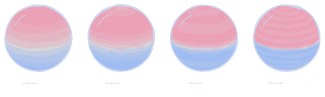
Halving the error costs $4\times$ the shells. The overshoot at the edge never goes away: it stays at $\approx1.18\,V_0$ for every $\ell_{\max}$ and only gets narrower (Gibbs).
Recipe: pick $\ell_{\max}\approx\frac{\pi}{\Delta\theta}$ from the smallest feature, then check the dropped tail $\sum_{\ell>\ell_{\max}}E_{\ell}$ against the tolerance. Smooth data converges fast; jumps converge slowly and never pointwise.
Why Cut at a Full Shell
“Full shell” means the cut is in $\ell$ only: every kept $\ell$ keeps all $2\ell+1$ values of $m$. The alternative is an $m$-cut: also drop every $|m|>M$.
Why not cut in $m$? Previously, rotations about $x$ and $y$ shuffle the $m$’s within a shell without changing $\hat{\Lambda}$. In symbols, a rotation $\hat{R}$ commutes with $\hat{\Lambda}$, so it can’t move a ket out of its shell:
$$ \begin{align*} \hat{\Lambda}\big(\hat{R}\ket{\ell m}\big)&=\hat{R}\,\hat{\Lambda}\ket{\ell m}\\ &=-\ell(\ell+1)\big(\hat{R}\ket{\ell m}\big)\\ \implies\hat{R}\ket{\ell m}&=\sum_{m'=-\ell}^{\ell}\ket{\ell m'}\mel{\ell m'}{\hat{R}}{\ell m} \end{align*} $$So $\hat{R}\hat{P}_{\ell}=\hat{P}_{\ell}\hat{R}$ for every shell, and summing over $\ell\leq\ell_{\max}$ gives $\hat{R}\hat{T}_{\ell_{\max}}=\hat{T}_{\ell_{\max}}\hat{R}$. Truncate-then-rotate is rotate-then-truncate: the blur doesn’t care where $z$ points.
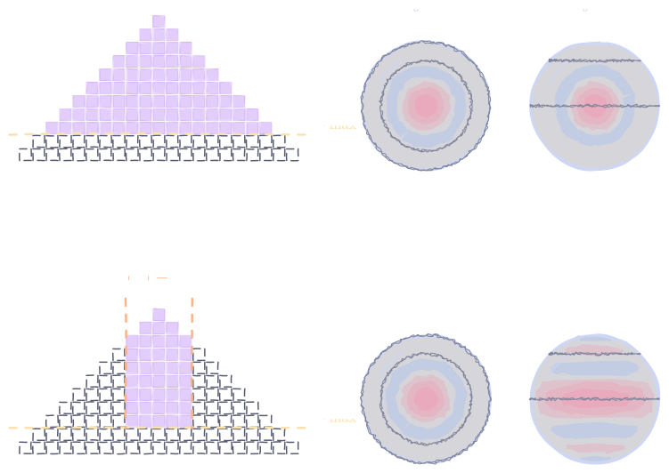
An $m$-cut keeps the single projectors $\ket{\ell m}\bra{\ell m}$ only for $|m|\leq M$. Those commute with $\hat{L}_z$ alone, i.e. with rotations about $z$. Previously, picking a $z$-axis was a free choice; an $m$-cut makes that choice show up in the answer. Previously, $m$ counts wavelengths around a circle of latitude. That circle has circumference $2\pi\sin\theta$, so the finest detail along $\psi$ (as an arc on the unit sphere) is
$$ \Delta s_{\psi}\approx\frac{\pi\sin\theta}{M} $$Near the poles $\sin\theta\to0$, so a small $M$ resolves everything. At the equator it takes $M\approx\ell_{\max}$. Same spot, different blur: with $\ell_{\max}=8$, full shells blur a spot at the pole and a spot on the equator identically; adding $|m|\leq2$ leaves the pole spot alone (only $m=0$ is nonzero at the pole, since $P_{\ell}^{|m|}(\cos\theta)\propto\sin^{|m|}\theta$) and smears the equator spot along the equator.
Other Geometries
Previously, the sphere’s modes came from its two boundary conditions: periodicity in $\psi$ gave $m$, finiteness at the poles gave $\ell$. What changes for a different boundary? The coordinates that fit it, the operator, and so the family of modes. The moves stay the same.
Bessel Functions
Circular drumhead of radius $a$, clamped at the rim. A time-harmonic $u=U e^{-i\omega t}$ turns the wave equation into Helmholtz:
$$ \begin{align*} \hat{\nabla}^2U&=-k^2U\\ k&=\frac{\omega}{v} \end{align*} $$Polar coordinates $(\rho,\psi)$:
$$ \hat{\nabla}^2=\frac{1}{\rho}\partial_{\rho}(\rho\,\partial_{\rho})+\frac{1}{\rho^2}\partial_{\psi}^2 $$Previously, $\hat{\Lambda}=\frac{1}{\sin\theta}\partial_{\theta}(\sin\theta\,\partial_{\theta})+\frac{1}{\sin^2\theta}\partial_{\psi}^2$. Same shape with $\sin\theta\to\rho$, so the same tensor-product split, with $\hat{A}\to\frac{1}{\rho}\partial_{\rho}(\rho\,\partial_{\rho})$ and $\hat{W}\to\frac{1}{\rho^2}$.
$\psi$ slot: unchanged. $\braket{\psi}{m}=e^{im\psi}$, and periodicity gives $m\in\mathbb{Z}$.
$\rho$ slot, at fixed $m$:
$$ \hat{D}_m^{(\rho)}=\frac{1}{\rho}\partial_{\rho}(\rho\,\partial_{\rho})-\frac{m^2}{\rho^2} $$The same centrifugal barrier as before, $\frac{m^2}{\rho^2}$ instead of $\frac{m^2}{\sin^2\theta}$. Eigenvalue problem $\hat{D}_m^{(\rho)}R=-k^2R$. Multiply by $\rho^2$ and set $s=k\rho$:
$$ \left[s^2\partial_{s}^2+s\,\partial_{s}+s^2-m^2\right]R=0 $$This is Bessel’s equation. Solutions: $J_m(k\rho)$, and a second one that goes like $\rho^{-|m|}$ ($\ln\rho$ for $m=0$) at the center. Infinite at the center, so chuck it, same as $Q_{\ell}^{m}(\cos\theta)$.
Where does $k$ get quantized? The sphere had no edge, so $\ell$ came from finiteness. The drum has one:
$$ \begin{align*} U(a,\psi)&=0\\ \implies J_m(ka)&=0\\ \implies k_{mn}&=\frac{j_{mn}}{a} \end{align*} $$$j_{mn}$ is the $n$-th zero of $J_m$, with no closed form: $j_{01}\approx2.405$, $j_{11}\approx3.832$, $j_{21}\approx5.136$, $j_{02}\approx5.520$. On the sphere the eigenvalues were integers, $-\ell(\ell+1)$. Here $\frac{\omega_{mn}}{\omega_{01}}=1.59,\ 2.14,\ 2.30,\dots$ are not: the overtones aren’t harmonics, which is why a drum has no clear pitch.
Orthogonality, by the same argument as before, with weight $\rho$ instead of $\sin\theta$:
$$ \begin{align*} &\left(k_{mn'}^2-k_{mn}^2\right)\\ &\quad\times\int_{0}^{a}J_m(k_{mn}\rho)\,J_m(k_{mn'}\rho)\,\rho\,\mathrm{d}\rho\\ &\quad=\Big[\rho\Big(J_m(k_{mn'}\rho)\,\partial_{\rho}J_m(k_{mn}\rho)\\ &\qquad-J_m(k_{mn}\rho)\,\partial_{\rho}J_m(k_{mn'}\rho)\Big)\Big]_{0}^{a}\\ &\quad=0 \end{align*} $$$\rho=0$ kills the lower end and the clamp $J_m(k_{mn}a)=0$ kills the upper. On the sphere, $\sin\theta$ killed both.
Nodal lines: $|m|$ diameters from $\cos(m\psi)$ and $n-1$ circles from the zeros of $J_m$ inside the rim. Previously: $\ell-|m|$ latitude circles and $|m|$ meridians.
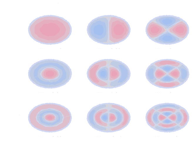
Laplace inside a cylinder: the same $\rho$ and $\psi$ modes, and the leftover coordinate $z$ gets one ODE per mode, $\partial_{z}^2Z=k_{mn}^2Z$, so $\sinh(k_{mn}z)$ and $\cosh(k_{mn}z)$. Previously, $r$ got $r^{\ell}$ and $r^{-(\ell+1)}$.
Mathieu Functions
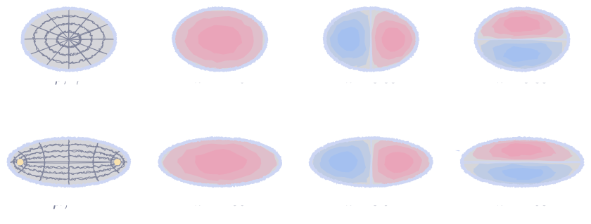
Squash the drum into an ellipse with foci at $(\pm d,0)$. Elliptic coordinates $(\mu,\nu)$:
$$ \begin{align*} x&=d\cosh\mu\,\cos\nu\\ y&=d\sinh\mu\,\sin\nu \end{align*} $$$\mu=\text{const}$: confocal ellipses ($\mu=0$ is the segment between the foci). $\nu=\text{const}$: confocal hyperbolas. $\nu$ is periodic, like $\psi$. Far away, $\cosh\mu\approx\sinh\mu\approx\frac{e^{\mu}}{2}$, so $d\cosh\mu\approx d\sinh\mu\to\rho$ and $\nu\to\psi$: polar coordinates come back.
Laplacian:
$$ \hat{\nabla}^2=\frac{1}{d^2\left(\sinh^2\mu+\sin^2\nu\right)}\left(\partial_{\mu}^2+\partial_{\nu}^2\right) $$Helmholtz, multiplied through by $d^2\left(\sinh^2\mu+\sin^2\nu\right)$, with $\sinh^2\mu=\frac{\cosh2\mu-1}{2}$ and $\sin^2\nu=\frac{1-\cos2\nu}{2}$:
$$ \begin{align*} \left(\partial_{\mu}^2+\partial_{\nu}^2\right)U&=-k^2d^2\left(\sinh^2\mu+\sin^2\nu\right)U\\ &=-\frac{k^2d^2}{2}\left(\cosh2\mu-\cos2\nu\right)U\\ &=-2q\left(\cosh2\mu-\cos2\nu\right)U\\ q&=\frac{k^2d^2}{4} \end{align*} $$Separate, $U=R(\mu)N(\nu)$, with separation constant $\alpha$:
$$ \begin{align*} \partial_{\nu}^2N+\left(\alpha-2q\cos2\nu\right)N&=0\\ \partial_{\mu}^2R-\left(\alpha-2q\cosh2\mu\right)R&=0 \end{align*} $$These are Mathieu’s equation and the modified Mathieu equation.
What’s new? $q$ contains $k$. On the sphere and on the drum, the $\psi$ eigenvalue $m^2$ never knew the frequency. Here the angular eigenvalue $\alpha$ depends on $k$ through $q$, so the angular modes change shape with frequency: the two slots no longer come apart completely.
$\nu$ slot: $N(\nu+2\pi)=N(\nu)$ only for special $\alpha$. $\alpha=\alpha_n^{c}(q)$: even solutions $\mathrm{ce}_n(\nu,q)$. $\alpha=\alpha_n^{s}(q)$: odd solutions $\mathrm{se}_n(\nu,q)$. At $q=0$: $\partial_{\nu}^2N+\alpha N=0$, so $\mathrm{ce}_n=\cos n\nu$, $\mathrm{se}_n=\sin n\nu$ and $\alpha=n^2$. Previously, the $\psi$ slot: $e^{im\psi}$ with eigenvalue $m^2$.
$\mu$ slot: the clamp at the rim $\mu=\mu_0$ picks $q$, and with it $k=\frac{2\sqrt{q}}{d}$:
$$ R_n(\mu_0,q)=0 $$Both conditions have to hold at the same $q$, so the $\nu$ and $\mu$ problems get solved together, not one after the other.
Degeneracy splits. On the circle, $J_m(ka)=0$ doesn’t care whether the $\psi$ part is $\cos m\psi$ or $\sin m\psi$: same $k$, a degenerate pair (a rotation turns one into the other). The ellipse has no rotation symmetry, $\alpha_n^{c}(q)\neq\alpha_n^{s}(q)$ for $q>0$, so $\mathrm{ce}_n$ and $\mathrm{se}_n$ ring at different $k$. Computed numerically, for an ellipse with the unit circle’s area (semi-axes $1.3$ and $\frac{1}{1.3}$): the pair at $k=3.83$ splits into $3.54$ (nodal line cutting the long axis in half) and $4.53$ (nodal line along the long axis). The fundamental moves from $2.40$ to $2.56$.
Hermite-Gaussian Functions
2D quantum harmonic oscillator, natural units:
$$ \hat{H}=-\frac{1}{2}\left(\partial_{x}^2+\partial_{y}^2\right)+\frac{1}{2}\left(x^2+y^2\right) $$Tensor-product split, as for $\hat{\Lambda}$:
$$ \begin{align*} \hat{H}&=\left(\hat{h}\otimes\hat{1}\right)+\left(\hat{1}\otimes\hat{h}\right)\\ \hat{h}&=-\frac{1}{2}\partial_{x}^2+\frac{1}{2}x^2 \end{align*} $$Previously, $\hat{\Lambda}=(\hat{A}\otimes\hat{1})-(\hat{W}\otimes\hat{L}_z^2)$: the $\theta$ slot carried $\hat{W}=\frac{1}{\sin^2\theta}$, which is why $\hat{D}_m$ depended on $m$. Here there is no cross term. Each slot is diagonalized alone, the labels never talk, and $E=E_{n_x}+E_{n_y}$.
1D slot, $\hat{h}\phi=E\phi$. Peel off the Gaussian, $\phi=h(x)\,e^{-x^2/2}$:
$$ \begin{align*} &\partial_{x}^2\phi=\left(\partial_{x}^2h-2x\,\partial_{x}h-h+x^2h\right)e^{-x^2/2}\\ &-\frac{1}{2}\partial_{x}^2\phi+\frac{1}{2}x^2\phi\\ &\quad=\left(-\frac{1}{2}\partial_{x}^2h+x\,\partial_{x}h+\frac{1}{2}h\right)e^{-x^2/2}\\ &\implies\partial_{x}^2h-2x\,\partial_{x}h+(2E-1)h=0 \end{align*} $$The $\frac{1}{2}x^2h$ from the potential cancels the $-\frac{1}{2}x^2h$ from the second derivative.
Power series, $h=\sum_k a_kx^k$:
$$ a_{k+2}=\frac{2k-(2E-1)}{(k+2)(k+1)}\,a_{k} $$If it never stops, $\frac{a_{k+2}}{a_k}\to\frac{2}{k}$, the same ratio as $e^{x^2}=\sum_j\frac{x^{2j}}{j!}$. Then $\phi\sim e^{x^2}e^{-x^2/2}=e^{x^2/2}$: not normalizable. Previously, the Legendre series diverged at the poles until $\lambda=\ell(\ell+1)$ cut it off. Same fix: stop the series at $k=n$ (and kill the other parity, as with $a_1=0$ before):
$$ \begin{align*} 2n-(2E-1)&=0\\ \implies E_n&=n+\tfrac{1}{2} \end{align*} $$The polynomial that’s left is the Hermite polynomial $H_n(x)$.
The 2D modes and energies:
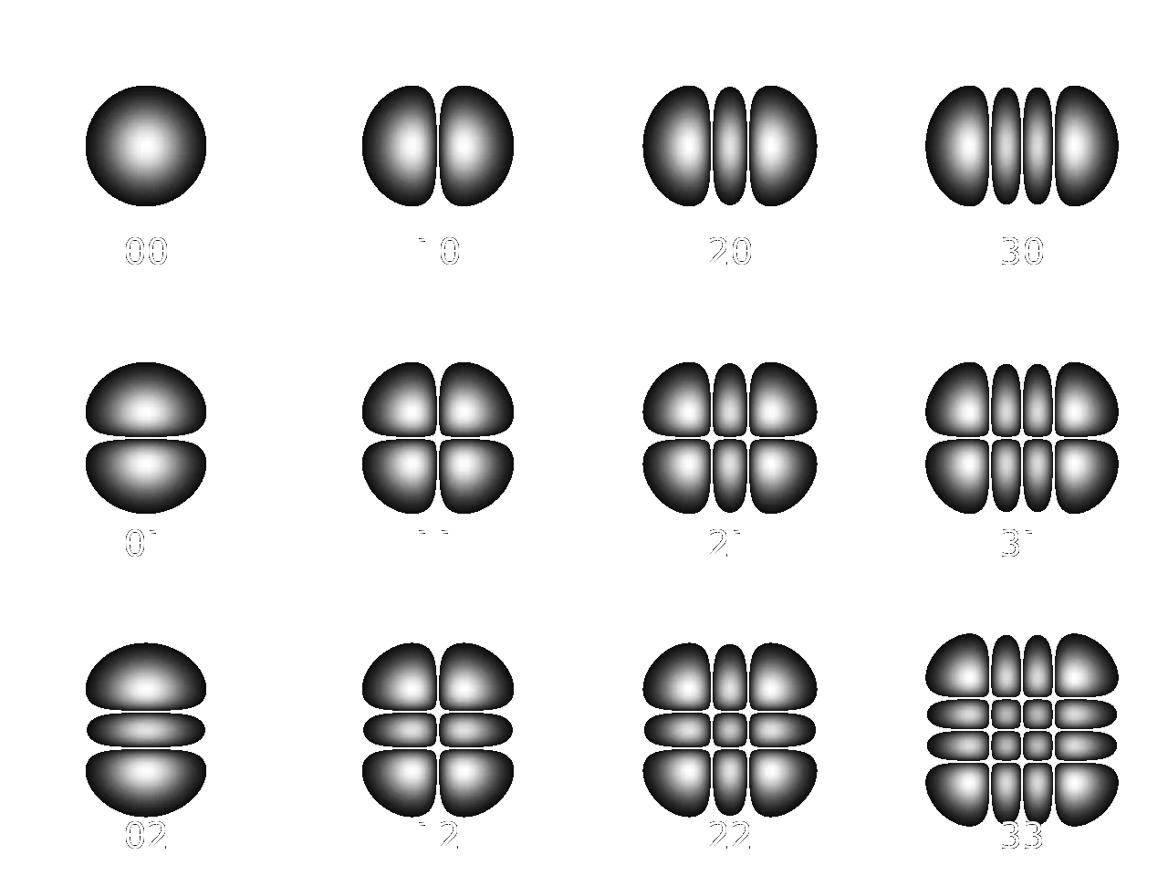
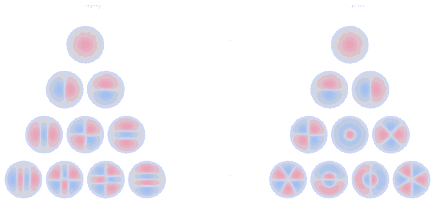
$$ \begin{align*} \phi_{n_xn_y}(x,y)&=H_{n_x}(x)\,H_{n_y}(y)\,e^{-(x^2+y^2)/2}\\ E&=n_x+n_y+1 \end{align*} $$Nodal lines: $n_x$ vertical and $n_y$ horizontal, a checkerboard of lobes. Shell $N=n_x+n_y$ holds $N+1$ degenerate modes. The potential is round, so rotations about the origin shuffle modes within a shell, as rotations shuffled $m$ within an $\ell$-shell.
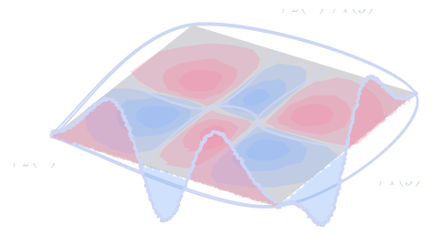
Laser beams: the paraxial wave equation for a beam along $z$, $\nabla_{\perp}^2u+2ik\,\partial_{z}u=0$, has the form of the 2D Schrödinger equation with $z$ playing time. The Hermite-Gaussian patterns are the $\mathrm{TEM}_{n_xn_y}$ transverse modes of a laser cavity: they keep their shape as they propagate, widening with the beam and picking up a phase proportional to $n_x+n_y+1$ (the Gouy phase). The shell index again.

Spheroidal Wave Functions
Stretch the sphere into a cigar. Prolate spheroidal coordinates $(\xi,\eta,\psi)$, foci at $z=\pm d$, with $\rho$ the distance from the $z$-axis:
$$ \begin{align*} \rho&=d\sqrt{(\xi^2-1)(1-\eta^2)}\\ z&=d\,\xi\eta \end{align*} $$$\xi\geq1$ and $-1\leq\eta\leq1$. $\xi=\text{const}$: prolate spheroids. $\eta=\text{const}$: hyperboloids. $\psi$ is untouched. Far away, $\xi\gg1$: $d\xi\to r$ and $\eta\to\cos\theta$. Spherical coordinates come back.
Laplacian:
$$ \begin{align*} \hat{\nabla}^2&=\frac{1}{d^2(\xi^2-\eta^2)}\Big[\partial_{\xi}(\xi^2-1)\partial_{\xi}\\ &\qquad+\partial_{\eta}(1-\eta^2)\partial_{\eta}\Big]\\ &\quad+\frac{1}{d^2(\xi^2-1)(1-\eta^2)}\partial_{\psi}^2 \end{align*} $$Helmholtz, multiplied through by $d^2(\xi^2-\eta^2)$, with $\braket{\psi}{m}=e^{im\psi}$ in the $\psi$ slot and
$$ \frac{\xi^2-\eta^2}{(\xi^2-1)(1-\eta^2)}=\frac{1}{1-\eta^2}+\frac{1}{\xi^2-1} $$Separate, $U=R(\xi)\,S(\eta)\,e^{im\psi}$, with separation constant $\lambda$:
$$ \begin{align*} &\partial_{\eta}\left[(1-\eta^2)\,\partial_{\eta}S\right]\\ &\quad+\left(\lambda-c^2\eta^2-\frac{m^2}{1-\eta^2}\right)S=0\\ &\partial_{\xi}\left[(1-\xi^2)\,\partial_{\xi}R\right]\\ &\quad+\left(\lambda-c^2\xi^2-\frac{m^2}{1-\xi^2}\right)R=0\\ &c=kd \end{align*} $$One equation on two ranges: $-1\leq\eta\leq1$ for the angular functions $S_{mn}(c,\eta)$, $\xi\geq1$ for the radial ones. $c=kd$ compares the focal distance with the wavelength.
Recognize it? At $c=0$, put $\eta=\cos\theta$. Previously, the $\theta$ equation:
$$ \begin{align*} &\frac{1}{\sin\theta}\partial_{\theta}(\sin\theta\,\partial_{\theta}S)\\ &\quad+\left(\lambda-\frac{m^2}{\sin^2\theta}\right)S=0 \end{align*} $$So $S_{mn}(0,\cos\theta)=P_{n}^{|m|}(\cos\theta)$ and $\lambda=n(n+1)$. At $c=0$ the wave can’t tell the spheroid from a sphere.
At $c>0$, the extra $c^2\eta^2$ acts as a potential: the eigenvalue problem is
$$ \left[-\partial_{\eta}(1-\eta^2)\partial_{\eta}+\frac{m^2}{1-\eta^2}+c^2\eta^2\right]S=\lambda S $$The Legendre modes don’t diagonalize it: $\eta P_{n}^{|m|}(\eta)$ only reaches $P_{n\pm1}^{|m|}(\eta)$, so $\eta^2$ couples $n$ to $n\pm2$. Rediagonalize:
$$ S_{mn}(c,\eta)=\sum_{\ell\geq|m|}d_{\ell}^{mn}(c)\,P_{\ell}^{|m|}(\eta) $$Only $\ell-n$ even. The matrix is diagonal, $\ell(\ell+1)$, plus $c^2$ times a band ($\ell\leftrightarrow\ell\pm2$). Previously, we diagonalized $\hat{\Lambda}$ in $\ket{\ell m}$; now the operator has changed, so the basis gets rotated within each $m$-block. $m$ stays a good label because $\psi$ is untouched.
Large $c$: the potential $c^2\eta^2$ squeezes $S$ toward $\eta=0$. There $1-\eta^2\approx1$, and for $m=0$:
$$ -\partial_{\eta}^2S+c^2\eta^2S\approx\lambda S $$Rescale, $t=\sqrt{c}\,\eta$:
$$ \left(-\frac{1}{2}\partial_{t}^2+\frac{1}{2}t^2\right)S=\frac{\lambda}{2c}S $$That’s the oscillator from before, so $\frac{\lambda}{2c}=n+\frac{1}{2}$:
$$ \begin{align*} \lambda&\approx c\,(2n+1)\\ S_{0n}(c,\eta)&\approx H_n(\sqrt{c}\,\eta)\,e^{-c\eta^2/2} \end{align*} $$Numerically at $c=14$: $\lambda=13.2,\ 40.2,\ 66.0,\ 90.6$ against $c(2n+1)=14,\ 42,\ 70,\ 98$. Low $n$ fits best, since the approximation needs the mode to stay near $\eta=0$. Spheroidal functions interpolate: Legendre at $c=0$, Hermite-Gaussian as $c\to\infty$.
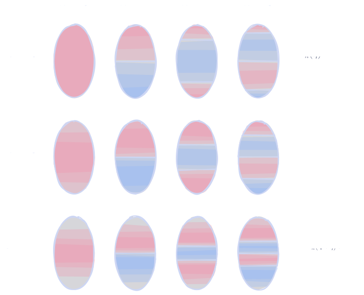
Oblate spheroids (a squashed sphere): $c\to ic$ flips the potential to $-c^2\eta^2$, which pushes $S$ toward the poles $\eta=\pm1$ instead.
Where they show up: waves scattering off or radiating from elongated bodies (antennas, needles); the $\mathrm{H}_2^{+}$ ion, whose two nuclei sit at the foci; and Slepian’s prolate spheroidal functions in signal processing, where the $S_{0n}$ are the band-limited signals most concentrated in a time window.
Laguerre Polynomials
$$ \hat{H}=-\frac{1}{2}\hat{\nabla}^2-\frac{1}{r} $$Previously, $\hat{\nabla}^2=\frac{1}{r^2}\partial_{r}(r^2\partial_{r})+\frac{1}{r^2}\hat{\Lambda}$ and $\mel{\ell m}{\hat{\Lambda}}{\Psi}=-\ell(\ell+1)\braket{\ell m}{\Psi}$. Sandwich $\hat{H}\ket{\Psi}=E\ket{\Psi}$ with $\bra{\ell m}$:
$$ \begin{align*} &\left[-\frac{1}{2r^2}\partial_{r}\left(r^2\partial_{r}\right)+\frac{\ell(\ell+1)}{2r^2}-\frac{1}{r}\right]\\ &\quad\times\braket{\ell m}{\Psi(r)}\\ &\quad=E\braket{\ell m}{\Psi(r)} \end{align*} $$The same radial operator as Laplace, plus a potential and an energy. $\frac{\ell(\ell+1)}{2r^2}$ is the centrifugal barrier again.
Peel off both ends. Near $r=0$ the barrier wins, and previously that gave $r^{\ell}$. Far away, $-\frac{1}{2}\partial_{r}^2\approx E$ with $E<0$ gives $e^{-\kappa r}$, $\kappa=\sqrt{-2E}$:
$$ \begin{align*} \braket{\ell m}{\Psi(r)}&=r^{\ell}e^{-\kappa r}\,u(s)\\ s&=2\kappa r \end{align*} $$What’s left for $u$:
$$ \begin{align*} &s\,\partial_{s}^2u+(2\ell+2-s)\,\partial_{s}u\\ &\quad+\left(\frac{1}{\kappa}-\ell-1\right)u=0 \end{align*} $$Power series, $u=\sum_kb_ks^k$:
$$ b_{k+1}=\frac{k+\ell+1-1/\kappa}{(k+1)(k+2\ell+2)}\,b_{k} $$If it never stops, $\frac{b_{k+1}}{b_k}\to\frac{1}{k}$, like $e^{s}$. Then the mode goes like $e^{-\kappa r}e^{2\kappa r}=e^{\kappa r}$: not normalizable. Same fix, third time. Stop the series at $k=n_r$:
$$ \begin{align*} \frac{1}{\kappa}&=n_r+\ell+1\equiv n\\ \implies E_n&=-\frac{\kappa^2}{2}\\ &=-\frac{1}{2n^2} \end{align*} $$The polynomial that’s left is the associated Laguerre polynomial $L_{n-\ell-1}^{2\ell+1}(s)$, with $s=\frac{2r}{n}$:
$$ \begin{align*} \Psi_{n\ell m}(r,\theta,\psi)&\propto\left(\frac{2r}{n}\right)^{\ell}e^{-r/n}\\ &\quad\times L_{n-\ell-1}^{2\ell+1}\!\left(\frac{2r}{n}\right)Y_{\ell m}(\theta,\psi) \end{align*} $$
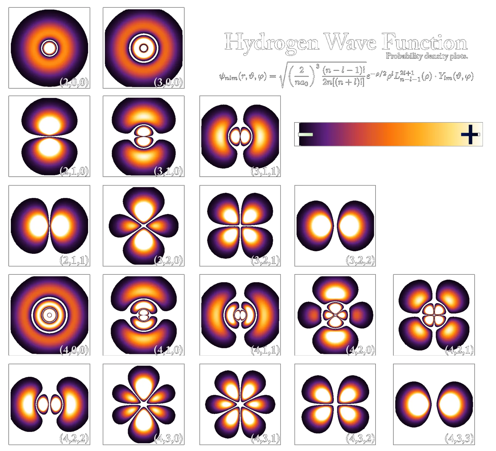

Nodes: $n-\ell-1$ spheres from the zeros of $L_{n-\ell-1}^{2\ell+1}$, plus the $\ell$ angular nodal surfaces of $Y_{\ell m}$ from before: $n-1$ in total.
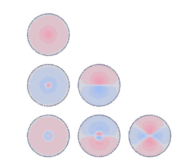
Degeneracy: $E$ depends on $n$ alone, and shell $n$ holds
$$ \sum_{\ell=0}^{n-1}(2\ell+1)=n^2 $$The same count as $(\ell_{\max}+1)^2$ in Truncation, with $\ell_{\max}=n-1$. Rotations explain the $2\ell+1$ within each $\ell$. The degeneracy across $\ell$ is special to $\frac{1}{r}$ (an extra conserved quantity, the Runge-Lenz vector).
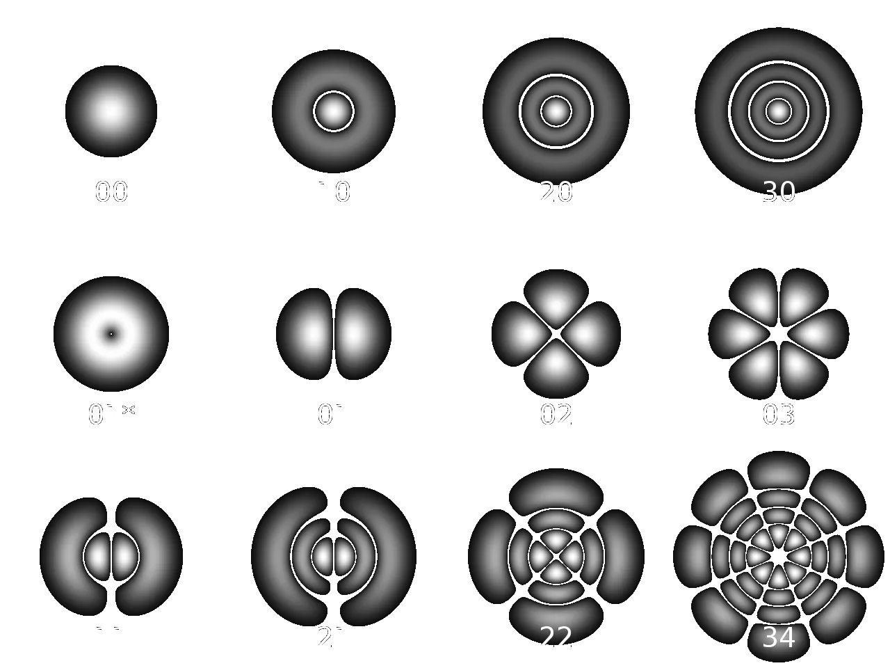
Laguerre-Gaussian: the 2D oscillator from before, in polar coordinates:
$$ \begin{align*} \hat{H}&=-\frac{1}{2}\left[\frac{1}{\rho}\partial_{\rho}(\rho\,\partial_{\rho})+\frac{1}{\rho^2}\partial_{\psi}^2\right]\\ &\quad+\frac{1}{2}\rho^2 \end{align*} $$$\psi$ slot: $e^{im\psi}$. $\rho$ slot: $-\frac{1}{2}\hat{D}_m^{(\rho)}+\frac{1}{2}\rho^2$, with $\hat{D}_m^{(\rho)}$ from the drum. Peel off $\rho^{|m|}$ at the center and $e^{-\rho^2/2}$ far away, and the series stops the same way:
$$ \begin{align*} \braket{\rho\,\psi}{p\,m}&=\rho^{|m|}L_p^{|m|}(\rho^2)\,e^{-\rho^2/2}\,e^{im\psi}\\ E&=2p+|m|+1 \end{align*} $$Same energies as the Hermite-Gaussians with $N=2p+|m|=n_x+n_y$. They are two bases of the same shells, the way $Y_{\ell m}$ about different $z$-axes are two bases of one $\ell$-shell. Shell $N=2$, with real $\psi$ parts:
$$ \begin{align*} &\left(1-\rho^2\right)e^{-\rho^2/2}\\ &\quad=-\frac{1}{4}\Big[H_2(x)+H_2(y)\Big]e^{-(x^2+y^2)/2}\\ &\rho^2\cos2\psi\,e^{-\rho^2/2}\\ &\quad=\frac{1}{4}\Big[H_2(x)-H_2(y)\Big]e^{-(x^2+y^2)/2}\\ &\rho^2\sin2\psi\,e^{-\rho^2/2}\\ &\quad=\frac{1}{2}H_1(x)\,H_1(y)\,e^{-(x^2+y^2)/2} \end{align*} $$In optics, Laguerre-Gaussian beams are the “donut” modes. The $e^{im\psi}$ makes them eigenkets of $\hat{L}_z$, so each photon carries orbital angular momentum $m\hbar$.

Poisson’s Equation
With a charge density $\rho(\vec{r})$:
$$ \hat{\nabla}^2\varphi=-\frac{\rho}{\varepsilon_0} $$Sandwich with $\bra{\ell m}$, as for Laplace:
$$ \begin{align*} &\left[\frac{1}{r^2}\partial_{r}\left(r^2\partial_{r}\right)-\frac{\ell(\ell+1)}{r^2}\right]\braket{\ell m}{\varphi(r)}\\ &\quad=-\frac{1}{\varepsilon_0}\braket{\ell m}{\rho(r)} \end{align*} $$The same radial operator, now driven: each mode is pushed only by its own piece of the charge. The modes still don’t talk.
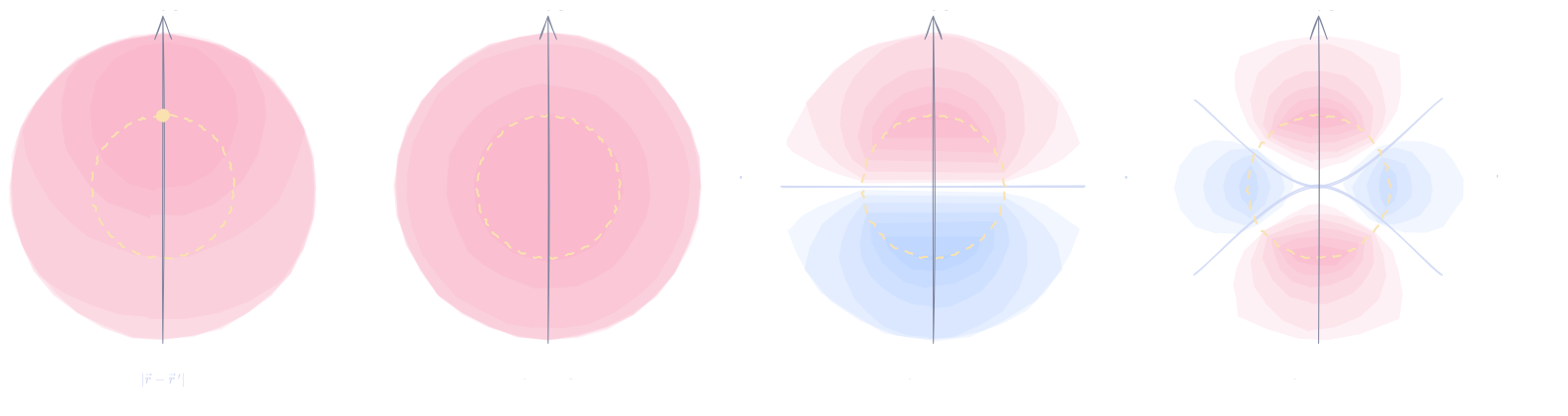
Point charge $q$ at $\vec{r}\,'=r'\hat{n}'$. Previously, $\braket{\hat{n}'}{\hat{n}}=\frac{\delta(\theta-\theta')}{\sin\theta}\,\delta(\psi-\psi')$. Insert the completeness of $\ket{\ell m}$:
$$ \begin{align*} \braket{\hat{n}}{\hat{n}'}&=\sum_{\ell m}\braket{\hat{n}}{\ell m}\braket{\ell m}{\hat{n}'}\\ &=\sum_{\ell m}Y_{\ell m}(\hat{n})\,Y_{\ell m}^*(\hat{n}') \end{align*} $$So $\rho=q\,\frac{\delta(r-r')}{r^2}\braket{\hat{n}}{\hat{n}'}$ has one coefficient per mode:
$$ \braket{\ell m}{\rho(r)}=q\,\frac{\delta(r-r')}{r^2}\,Y_{\ell m}^*(\hat{n}') $$Off the shell $r=r'$, the right side vanishes and it’s Laplace, with $r^{\ell}$ and $r^{-(\ell+1)}$ from before. Finite at $0$ inside, at $\infty$ outside, continuous at $r'$:
$$ \begin{align*} \braket{\ell m}{\varphi(r)}&=\frac{q}{\varepsilon_0}\,Y_{\ell m}^*(\hat{n}')\,C_{\ell}\,\frac{r_<^{\ell}}{r_>^{\ell+1}}\\ r_<&=\min(r,r')\\ r_>&=\max(r,r') \end{align*} $$The $\delta$ fixes $C_{\ell}$. Multiply by $r^2$ and integrate across $r=r'$; only the derivative jumps:
$$ \begin{align*} &r'^2\Big[\partial_{r}\braket{\ell m}{\varphi(r)}\Big]_{r'^-}^{r'^+}=-\frac{q}{\varepsilon_0}Y_{\ell m}^*(\hat{n}')\\ &\frac{q}{\varepsilon_0}Y_{\ell m}^*(\hat{n}')\,C_{\ell}\,r'^2\left(-\frac{\ell+1}{r'^2}-\frac{\ell}{r'^2}\right)\\ &\quad=-\frac{q}{\varepsilon_0}Y_{\ell m}^*(\hat{n}')\\ &\implies C_{\ell}=\frac{1}{2\ell+1} \end{align*} $$Sum the modes and compare with Coulomb, $\varphi=\frac{q}{4\pi\varepsilon_0|\vec{r}-\vec{r}\,'|}$:
$$ \begin{align*} \varphi(\vec{r})&=\frac{q}{\varepsilon_0}\sum_{\ell m}\frac{1}{2\ell+1}\frac{r_<^{\ell}}{r_>^{\ell+1}}\\ &\qquad\times Y_{\ell m}^*(\hat{n}')\,Y_{\ell m}(\hat{n})\\ \implies\frac{1}{|\vec{r}-\vec{r}\,'|}&=\sum_{\ell m}\frac{4\pi}{2\ell+1}\frac{r_<^{\ell}}{r_>^{\ell+1}}\\ &\qquad\times Y_{\ell m}^*(\hat{n}')\,Y_{\ell m}(\hat{n}) \end{align*} $$Charge on the $z$-axis: previously, pointing $z$ along the symmetry axis kills every $m\neq0$. With $Y_{\ell 0}^*(\hat{z})=\sqrt{\frac{2\ell+1}{4\pi}}$ and $Y_{\ell 0}(\hat{n})=\sqrt{\frac{2\ell+1}{4\pi}}P_{\ell}(\cos\theta)$:
$$ \frac{1}{|\vec{r}-r'\hat{z}|}=\sum_{\ell=0}^{\infty}\frac{r_<^{\ell}}{r_>^{\ell+1}}P_{\ell}(\cos\theta) $$Interpretation: the charge acts like boundary data on the sphere $r=r'$. Each mode is Laplace’s $r^{\ell}$ inside and $r^{-(\ell+1)}$ outside, and the charge is the kink that joins them.
Multipole expansion: for $r$ outside all the charge, $r_<=r'$ and $r_>=r$. Superposing point charges:
$$ \begin{align*} \varphi(\vec{r})&=\frac{1}{\varepsilon_0}\sum_{\ell m}\frac{1}{2\ell+1}\,\frac{q_{\ell m}}{r^{\ell+1}}\,Y_{\ell m}(\hat{n})\\ q_{\ell m}&=\int Y_{\ell m}^*(\hat{n}')\,r'^{\ell}\rho(\vec{r}\,')\,\mathrm{d}^3r' \end{align*} $$$\ell=0$ is the total charge, $\ell=1$ the dipole, $\ell=2$ the quadrupole. The $\ell$-th term dies as $r^{-(\ell+1)}$, so far away the lowest nonzero $\ell$ wins. Previously, from far away the sphere at $V_0\cos^2\theta$ looked like a point charge. Check at $\ell=0$, with $q_{00}=\frac{Q}{\sqrt{4\pi}}$ and $Y_{00}=\frac{1}{\sqrt{4\pi}}$:
$$ \frac{1}{\varepsilon_0}\cdot\frac{Q}{\sqrt{4\pi}}\cdot\frac{1}{r}\cdot\frac{1}{\sqrt{4\pi}}=\frac{Q}{4\pi\varepsilon_0r} $$Other PDEs
Same sandwich, different equation. In each one, $\bra{\ell m}$ turns the angular part into $-\ell(\ell+1)$, and the leftover coordinate gets one ODE per mode.
Heat on a spherical shell of radius $R$, diffusion constant $D$:
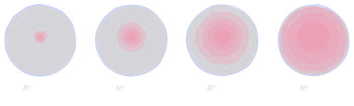
$$ \partial_{t}f=\frac{D}{R^2}\hat{\Lambda}f $$Sandwich:
$$ \begin{align*} \partial_{t}c_{\ell m}&=-\frac{D}{R^2}\ell(\ell+1)\,c_{\ell m}\\ \implies c_{\ell m}(t)&=c_{\ell m}(0)\,e^{-\ell(\ell+1)Dt/R^2} \end{align*} $$The leftover coordinate is $t$. High $\ell$ die first, so diffusion is a soft low-pass filter where truncation was a hard one. $\ell=0$ never decays (eigenvalue $0$), so the sphere settles to the average of the starting temperature. A hot spot at the north pole, $f(0)=\braket{\hat{n}}{\hat{z}}$, with $Y_{\ell m}^*(\hat{z})=\delta_{m0}\sqrt{\frac{2\ell+1}{4\pi}}$:
$$ \begin{align*} f(\theta,t)&=\sum_{\ell=0}^{\infty}\frac{2\ell+1}{4\pi}\,e^{-\ell(\ell+1)Dt/R^2}\\ &\qquad\times P_{\ell}(\cos\theta) \end{align*} $$At short times this is a Gaussian of angular width $\sigma=\frac{\sqrt{2Dt}}{R}$: the same $e^{-\ell(\ell+1)\sigma^2/2}$ as the smooth bump in Truncation.
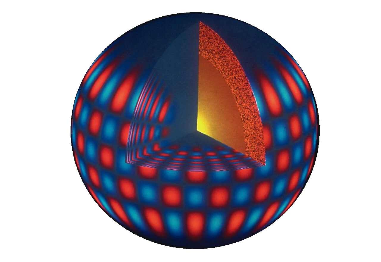
Waves on a sphere (a vibrating shell, the surface of a star), wave speed $v$:
$$ \begin{align*} \partial_{t}^2f&=\frac{v^2}{R^2}\hat{\Lambda}f\\ \implies c_{\ell m}(t)&\propto\cos\left(\omega_{\ell}t\right)\\ \omega_{\ell}&=\frac{v}{R}\sqrt{\ell(\ell+1)} \end{align*} $$Each shell rings at one frequency, all $2\ell+1$ values of $m$ together. Helioseismology labels the Sun’s oscillation modes by this $\ell$.
Helmholtz in 3D (sound in a spherical room, a particle in a ball):
$$ \begin{align*} &\left[\frac{1}{r^2}\partial_{r}\left(r^2\partial_{r}\right)-\frac{\ell(\ell+1)}{r^2}+k^2\right]\\ &\quad\times\braket{\ell m}{U(r)}=0 \end{align*} $$Solutions: the spherical Bessel function $j_{\ell}(kr)$, and a second one that blows up at $r=0$. Near the center the barrier beats $k^2$, and $j_{\ell}(kr)\propto(kr)^{\ell}$: Laplace’s $r^{\ell}$ from before. With $U=0$ on $r=R$, $k_{\ell n}=\frac{(n\text{-th zero of }j_{\ell})}{R}$. For $\ell=0$, $j_0(kr)=\frac{\sin kr}{kr}$, so $k_{0n}=\frac{n\pi}{R}$ exactly.
Any central potential $V(r)$: the same $Y_{\ell m}$, and the radial equation gets $\frac{\ell(\ell+1)}{2r^2}+V(r)$. Hydrogen was $V=-\frac{1}{r}$.
Conclusion: Diagonalize and Decouple
Everything in this series is one trick: find the operator the problem is secretly diagonal in, and the PDE falls apart into independent pieces.
The recipe, as it played out on the sphere: (1) Pick the operator acting on the coordinates the boundary data lives on: $\hat{\Lambda}$ on $(\theta,\psi)$. (2) Diagonalize it. The boundary conditions decide which modes are allowed: periodicity in $\psi$ gave $m$, finiteness at the poles gave $\ell$. (3) The leftover coordinate gets one ODE per mode, with the eigenvalue as a parameter: $r$, with $r^{\ell}$ and $r^{-(\ell+1)}$. (4) Fix the coefficients by projection: Fourier’s trick on $V$ gave $\braket{\ell m}{V}$.
References
- R. L. Herman, An Introduction to Mathematical Physics via Oscillations, Chapter 9, “Oscillations in Higher Dimensions,” University of North Carolina Wilmington (2012). PDF, licensed CC BY-NC-SA 3.0.
- F. W. J. Olver et al., eds., NIST Digital Library of Mathematical Functions, Chapter 10: Bessel Functions, Chapter 18: Orthogonal Polynomials, Chapter 28: Mathieu Functions and Hill’s Equation, and Chapter 30: Spheroidal Wave Functions.
- J. D. Jackson, Classical Electrodynamics, 3rd ed., Wiley (1999), Chapters 3 and 4.
- A. E. Siegman, Lasers, University Science Books (1986).
- N. K. Pavlis, S. A. Holmes, S. C. Kenyon, and J. K. Factor, “The development and evaluation of the Earth Gravitational Model 2008 (EGM2008),” Journal of Geophysical Research 117, B04406 (2012). doi:10.1029/2011JB008916
- Planck Collaboration, “Planck 2018 results. I. Overview and the cosmological legacy of Planck,” Astronomy & Astrophysics 641, A1 (2020). doi:10.1051/0004-6361/201833880, arXiv:1807.06205
- D. Slepian and H. O. Pollak, “Prolate spheroidal wave functions, Fourier analysis and uncertainty – I,” Bell System Technical Journal 40, 43–63 (1961). doi:10.1002/j.1538-7305.1961.tb03976.x
- L. Allen, M. W. Beijersbergen, R. J. C. Spreeuw, and J. P. Woerdman, “Orbital angular momentum of light and the transformation of Laguerre-Gaussian laser modes,” Physical Review A 45, 8185 (1992). doi:10.1103/PhysRevA.45.8185
<EOF>
We started by treating functions on a sphere as vectors and ended up with drums, lasers, hydrogen, and heat, all from diagonalizing one operator and letting the PDE fall apart into independent pieces. Hopefully, the next time a $Y_{\ell m}$ shows up, we both know what the hell we’re looking at. This concludes my blog post series on spherical harmonics.