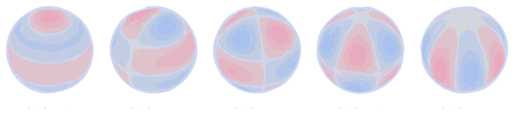
This series started as a note for my understanding of Spherical Harmonics, so that I can always revisit this as a reference and understand what the hell I’m looking at. That’s the chief reason. I really like to think of it from a physics pov, so I’m just gonna go with that.
There are a few other reasons, though. Spherical harmonics usually get handed to us as a finished formula that we’re supposed to trust, and I wanted to derive every piece ab initio instead: where $\ell$ and $m$ come from, why the normalization constant looks the way it does, and why the basis is orthogonal in the first place. I also have a taste for what I call low entropy expressions, ones that are factored so that their physical meaning is immediately clear, and spherical harmonics turned out to be a great place to practice that. And the trick at the heart of all of this (diagonalize, then decouple) isn’t just a sphere thing. It shows up in drumheads, laser modes, the hydrogen atom, maps of the cosmic microwave background, and Earth’s gravity field, so it’s worth understanding properly at least once.
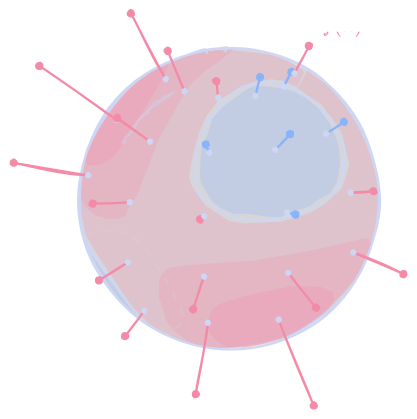
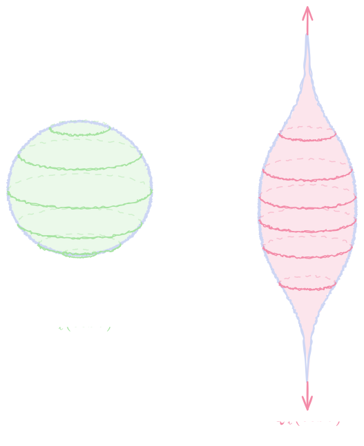
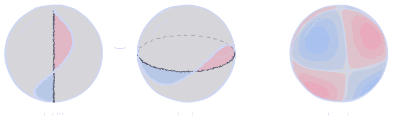
I believe that art is a great way to communicate science, so I tried to really do the visualizations well. Every figure in this series is drawn in a hand-sketched style, but computed from the actual math, so the shapes are the real ones. The colors mean something: red is $+$, blue is $-$, and anything hidden behind a surface is dashed and faded.
I also want this to be clear to whoever reads it, not just future me. The only prerequisites are some linear algebra and calculus. I use Dirac (bra-ket) notation throughout, and every new idea gets introduced right where it’s needed. Each post builds on the last one, so it’s best read in order.
Goal
We want to be able to decompose any function on the surface of a sphere into a summation of eigenbases. The sphere radius here is arbitrary and not super important for the purposes of our pedagogy. This follows from the fact that the eigenbases, or “modes” of a sphere, are completely independent of the radius of that sphere; which makes sense because the “shape” or “curvature” of the sphere is pretty much completely independent of a sphere’s radius.
Some Initial Terminology
Vectors and functions, as well as the operations between them, are totally interchangeable. This is not mathematically rigorous at all… so there is probably some edge case where this isn’t true, but humor me for a minute. We can decompose vectors into functional forms as follows:
Internalizing these beasties will allow us to truly understand how spherical harmonics work and how we can make money on them.
Making Money on Ts
Functions on a Sphere Are Vectors
Just really want to drive this point home. Functions on a sphere are synonymous with vectors and can be quantized as an expansion in the spherical eigenbasis! Suppose we have an arbitrary function $\ket{f}$ on a sphere. How is it characterized?
In other words, $\ket{f}$ is characterized by the “action” that it takes on a normal vector, $\hat{n}$ pointing outward from the sphere! The values $f(\hat{n})$ are the continuous components of $\ket{f}$, the same way the $c_{i}$ are the discrete components of $\vec{v}$:
So… what’s a good basis for the sphere of $\ket{f}$? Using the principle of least sloth, we want the eigenvectors of some operator (call it $\hat{\Lambda}$) so that we can diagonalize $\hat{\Lambda}$ in its eigenbasis and have the eigenkets that expand $\ket{f}$!
Since we deal with Laplace’s equation in E&M pretty frequently, a good choice for $\hat{\Lambda}$ is $r^2$ times the angular term of $\hat{\nabla}^2=\frac{1}{r^2}\partial_{r}(r^2\partial_{r})+\frac{1}{r^2}\hat{\Lambda}$. As stated previously, since the eigenbasis itself is independent of $R$, we may discard the radial part of $\hat{\nabla}^2$. For a sphere of radius $R$, $\frac{1}{R^2}\hat{\Lambda}$ is the “surface Laplacian,” which has the same eigenfunctions as $\hat{\Lambda}$, times the scale factor of $\frac{1}{R^2}$ for the eigenvalues.
So, looking at this guy, what does it actually measure?
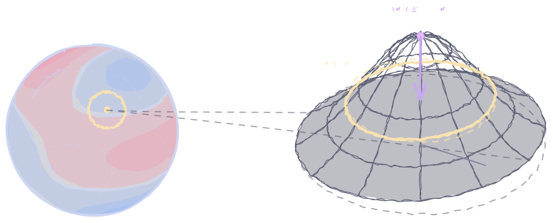
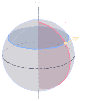
Claim: At each point on the spherical surface, $\langle \hat n|\hat\Lambda|f\rangle$ measures how much the average of $f(\hat{n}')$ over an infinitesimal circle around $\hat n$ exceeds $f(\hat n)$ itself. This is explained in more detail below, but the short version is $\left<f \right> -f \approx \frac{\varepsilon^2}{4}\mel{\hat{n}}{\hat{\Lambda}}{f}$.
Proof.
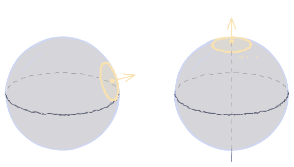
Consider a small, geodesic patch with radius $\varepsilon$ centered at the point containing $\hat{n}$. Then,
$$
\begin{align*}
&\left< f \right>_{\varepsilon}(\hat{n})\\
&\quad=\frac{1}{2\pi}\int_{0}^{2\pi} f(\hat{n}'(\varepsilon,\psi')) \,\mathrm{d}\psi'.
\end{align*}
$$
so that $\left< f \right>_{\varepsilon}(\hat{n})=g(\varepsilon)$ and $g(0)=\left< f \right>_{\text{pole}}=f(\text{pole})$.
Indeed, it is valid to conclude that $\varepsilon$, which we initially defined as the small radius in an arbitrary geodesic patch (which is also equal to the polar angle, $\theta$, between $\hat{n}$ and $\hat{n}'$ within the integral) is equivalent to the same variation in $\theta$ measured from the north pole (which is measured by $g$). This follows from the rotational invariance of the sphere, since you can just rotate the sphere and define $\hat{n}$ as the “new” north pole… which means that $g(0)=f(\hat{n})$.
$Y_{\ell m}$ is just another way to write “components of basis $\ket{\ell m}$ for all $\hat{n}$ on the sphere”.
Where $\ell$ and $m$ Come From
I just asserted $\hat{\Lambda}\ket{\ell m} = -\ell(\ell+1)\ket{\ell m}$. Let’s verify this is the case ab initio by formulating the eigenvalue problem as follows:
The minus sign is because $\mel{f}{\hat{\Lambda}}{f} \leq 0$, which follows from integrating by parts (not shown). A more hand-wavy explanation: on a closed sphere, $f$ must have a global maximum, and there it sits at or above its neighbors’ average. Therefore, $\hat{\Lambda}$ can’t push $f$ further in its own direction. Hence $\lambda$ itself must be $\geq 0$.
The third line where we pull $\hat{\Lambda}$ out of the braket would ordinarily be a mathematical tragedy, but it turns out there are a subset of operators for which you can pull the operator outside and let it act directly on the scalar function with no penalties. This is usually the case if the operator has a differential/multiplication representation in the basis defined by the bra, a principle known as structural locality. A convenient table for Hermitian observables is shown below (in natural units):
Operator
Shorthand in position basis
Position ($\hat{x}$)
$\langle x \vert \hat{x} \vert f \rangle = \hat{x}\,\langle x \vert f \rangle = x\,f(x)$
Function of position ($V(\hat{x})$)
$\langle x \vert V(\hat{x}) \vert f \rangle = V(\hat{x})\,\langle x \vert f \rangle = V(x)\,f(x)$
Momentum ($\hat{p}$)
$\langle x \vert \hat{p} \vert f \rangle = \hat{p}\,\langle x \vert f \rangle = -i\,\partial_{x}f(x)$
Momentum, 3D ($\hat{\vec{p}}$)
$\langle \vec{r} \vert \hat{\vec{p}} \vert f \rangle = \hat{\vec{p}}\,\langle \vec{r} \vert f \rangle = -i\vec{\nabla}f(\vec{r})$
Laplacian ($\hat{\nabla}^2=-\hat{p}^2$)
$\langle \vec{r} \vert \hat{\nabla}^2 \vert f \rangle = \hat{\nabla}^2\,\langle \vec{r} \vert f \rangle = \nabla^2 f(\vec{r})$
$\langle x \vert \hat{H} \vert f \rangle = \hat{H}\,\langle x \vert f \rangle = \left[-\frac{1}{2\mu}\partial_{x}^2+V(x)\right]f(x)$
Polar coordinate ($\cos\hat{\theta}$)
$\langle \hat{n} \vert \cos\hat{\theta} \vert f \rangle = \cos\hat{\theta}\,\langle \hat{n} \vert f \rangle = \cos\theta\,f(\theta,\psi)$
$z$-angular momentum ($\hat{L}_z$)
$\langle \hat{n} \vert \hat{L}_z \vert f \rangle = \hat{L}_z\,\langle \hat{n} \vert f \rangle = -i\,\partial_{\psi}f(\theta,\psi)$
Angular Laplacian ($\hat{\Lambda}=-\hat{L}^2$)
$\langle \hat{n} \vert \hat{\Lambda} \vert f \rangle = \hat{\Lambda}\,\langle \hat{n} \vert f \rangle = \left[\frac{1}{\sin\theta}\partial_{\theta}(\sin\theta\,\partial_{\theta})+\frac{1}{\sin^2\theta}\partial_{\psi}^2\right]f(\theta,\psi)$
$\theta$-operator at fixed $m$ ($\hat{D}_m$)
$\langle \theta \vert \hat{D}_m \vert f \rangle = \hat{D}_m\,\langle \theta \vert f \rangle = \left[\frac{1}{\sin\theta}\partial_{\theta}(\sin\theta\,\partial_{\theta})-\frac{m^2}{\sin^2\theta}\right]f(\theta)$
We can now see that we need to solve the PDE in $Y$ and determine the eigenvalue $\lambda$. There is also the question of how we’re actually going to express the original function, $f$, as a summation over the eigenbasis $\ket{\ell m}$, implying summation indices $\ell$ and $m$. Where exactly do these discretization indices/quantum numbers come from? Spoiler alert: We are going to use the fact that $Y$ is periodic-continuous to get $m$ and finite at the poles to get $\ell$.
Separation of Variables
Let’s use separation of variables to solve for $Y$. We begin with the ansatz that $Y(\theta,\psi) = \Theta(\theta)\Phi(\psi)$. Plug in, multiply by $\frac{\sin^2\theta}{\Theta\Phi}$, and rearrange:
Uniqueness implies $\Phi(\psi + 2\pi) = \Phi(\psi)$, so $e^{2\pi i m} = 1 (m \in \mathbb{Z})$. This is our first quantum number! We intentionally avoided $-m^2$ because then $\Phi = e^{\pm k\psi}$, which grows/decays monotonically and thus cannot be periodic-continuous.
The $\theta$ Equation in Nicer Variables
Apply the same separation of variables technique to $Y$, setting the LHS equal to $m^2$, and dividing by $\sin^2\theta$:
The general solution to the plain Legendre equation follows a recurrence relation from the power series ansatz $\Theta(x)=\sum_{n=0}^{\infty}a_{n}x^n$ where $a_{n+2}=\frac{n(n+1)-\lambda}{(n+2)(n+1)}a_{n}$. However, this diverges at $|x|=1$. Fix: set $\lambda=\ell(\ell+1)$ for some $\ell \in \{0, 1, 2, \dots\}$, causing the recurrence numerator to vanish at $n=\ell$, causing $a_{n \ge \ell+2}=0$. Another caveat: you must also set $a_{1}=0$ so all the odd coefficients die immediately (you could have also fixed the even coefficients to zero).
This leads to the ODE $[\partial_{x}(1-x^2)\partial_{x} + \ell(\ell+1)]\Theta = 0$, which also simultaneously gives $\lambda=\ell(\ell+1)$. The solutions are the Legendre polynomials:
Which have linear combinations of the associated Legendre functions, $P_{\ell}^m(x)$ and $Q_{\ell}^m(x)$, as solutions… except $Q_{\ell}^{m}(x)$ is ill-defined at $|x|=1$, so chuck it! And so, we have:
Okay, that was a lot of math. The takeaway is that each eigenket $\ket{\ell m}$ is a tensor product of a distinct pair of modes, each an eigenket of its own Hermitian 1D operator: the $m$-mode $\ket{m}=e^{im(\cdot)}$, eigenket of $\hat{L}_{z}$, and the Legendre mode $\ket{\ell}_{m}=P_{\ell}^{|m|}(\cos(\cdot))$, eigenket of $\hat{D}_m$. The “subscript $m$” just means the Legendre mode is for some fixed $m$. This makes sense because the associated Legendre function depends on your choice of $m$. More on $\hat{L}_{z}$ and $\hat{D}_{m}$ in the following section.
Claim: You can use $m \mapsto|m|$ for $\Theta$ because its ODE only has $m^2$. For all the masochists out there, you can still use the Legendre summation formula for $m \in [-\ell, 0]$ and get the same answer.
$N_{\ell m}$ is the normalization constant fixed by the inner product of eigenkets. We will come up with a concrete way to calculate $N_{\ell m}$ once we introduce $\hat{L}_{z}$ and $\hat{D}_{m}$ and discuss some additional properties of our chosen spherical basis that may be of use.
Introducing $\hat{L}_{z}$ and $\hat{D}_{m}$
As mentioned previously, our chosen spherical eigenbasis also serves as the eigenkets of $\hat{\Lambda}$, and it is also the tensor product of the Legendre and $m$-modes $(\ket{\ell m}\equiv\ket{\ell}_{m} \otimes \ket{m})$ with their own respective quantum numbers. But what operators do those individual modes correspond to? And is there any relationship between those operators and $\hat{\Lambda}$? In this section, I hope to answer those questions with fidelity.
Understanding $\bra{\hat{n}}$
First, let’s closely examine the vector $\bra{\hat{n}}$. It’s rather odd to have a unit-norm vector as a label within a bra (or ket for that matter). In fact, it’s something that I hadn’t seen before up until writing this (the benefits of making ts up as I go 😋). So what does $\bra{\hat{n}}$ really mean? Just like the eigenbasis $\ket{\ell m}$, $\bra{\hat{n}}$ is also just a tensor product of the input coordinate system:
This is important to keep in mind, since it turns out that $\bra{\theta \psi}$ serves as a basis for the dual space of $\ket{\ell m}$.
Tensor-Product Decomposition of $\hat{\Lambda}$
Now, let’s return back to our old friend $\hat{\Lambda}$. It turns out that any operator in a tensor-product Hilbert space can be expressed as a sum of tensor products of operators in each subspace, and we can use this fact to get $\hat{\Lambda}$ into a lower entropy form. Whenever I say “low entropy” in the context of problem-solving, I’m usually referring to an expression that is factored/structured in a certain way so that its physical meaning is immediately clear.
This pedagogical approach ties into how I viewed circuit theory in undergrad… essentially, it’s possible to convert any circuit into a matrix (even if it’s nonlinearly defined in the case of microelectronics, as the relationships are still linear), but the raw output of these matrices are usually unorganized as some kind of massive polynomial ratio where the physical intuition is lost and it’s not trivial to make approximations. As such, solving those kinds of systems usually has the tradeoff between speed and explainability.
So which half of $\bra{\theta \psi} \equiv \bra{\theta}\otimes\bra{\psi}$ actually reads $\hat{A}$ and $\hat{W}$? When it comes to formulating tensor products as an “action” on an operator, you can think of each sub-ket/sub-bra combo as “slotting” one of the operators in place. Mathematically, this is described as follows:
We can now sandwich $\hat{\Lambda}$ with the eigenket and eigenbra of the space:
$$
\mel{\theta \psi}{\hat{\Lambda}}{\ell m}
$$
But isn’t this just $-\lambda Y = -\ell(\ell+1) Y$? Why are we reinventing the wheel? Good question. The main purpose is to use this tensor-product-decomposed form of $\Lambda$ to provide more insight into the structure of $Y$ (the low entropy form I was describing earlier). We proceed as follows:
Notice that we have three slotted operators (well, technically four if you include the identity, but who gaf): $\hat{A}$, $\hat{W}$, $\partial_{\psi}^2$. Our job is to deal with these beasties one by one. Let’s deal with $\partial_{\psi}^2$ first, since it already contains another, somewhat-well-known operator, encoded inside:
Interpretation: $\ket{m}$ is an eigenket of $\partial_{\psi}^2$ with eigenvalue $-m^2$ (recall that $-m^2$ was our separation constant when we were doing separation of variables). We can use this to find the operator that is an eigenket of $\partial_{\psi}$ (tired of eigenvalue problems yet?). Since $\partial_{\psi}\ket{m}=im\ket{m}$, we have $-i\partial_{\psi}\ket{m}=m \ket{m}$. Call the left-acting operator $\hat{L}_z$:
It turns out that $\hat{L}_{z}$ is a well-known Hermitian operator, the angular momentum operator. It can also be thought of as the canonical operator that generates rotations about $z$:
Since $\partial_{\psi}^2=-\hat{L}_z^2$, we have $\hat{\Lambda}=(\hat{A}\otimes\hat{1})-(\hat{W}\otimes\hat{L}_z^2)$. Since $\hat{L}_{z}^2$ is the only operator slotted into $\bra{\psi}$, my claim is that the eigenkets of $\hat{L}_z$ span the entire $\bra{\psi}$ sub-space (one of our coordinate labels in the spherical basis!).
Now, what about the two operators slotted into $\ket{\theta}$? Let’s plug the $\bra{\psi}$ sucker back in:
Why was I able to pull out $\hat{A}$ and $\hat{W}$? Just like before, it’s because of structural locality. Since $\hat{A}=\frac{1}{\sin\theta}\partial_{\theta}(\sin\theta\,\partial_{\theta})$ and $\hat{W}=\frac{1}{\sin^2\theta}$ are solely dependent on $\theta$, reading $\braket{\theta}{\ell}$ first and operating afterwards still yields the same result. In other words: if the operator’s variable matches the bra label, you can bring it out of the sandwich!
From the result above, we can see that the operators slotted into $\bra{\theta}$ can be further collapsed into a single operator acting on the Legendre mode (call it $\hat{D}_{m}$). The “subscript $m$” is there because, similar to the Legendre modes, $\hat{D}_m$ only exists after the $\psi$ slot has handed over its eigenvalue. In other words: different $m$-mode, different $\hat{D}_m$.
Now, re-sandwich this beasty with the Legendre mode:
This is literally the $\theta$ equation we already solved! So, $\ket{\ell}_m$ is the eigenket of $\hat{D}_m$ with eigenvalue $-\ell(\ell+1)$, and for each fixed $m$ the eigenkets of $\hat{D}_m$ span the entire $\theta$ slot (or the $\theta$ coordinate label). Finishing the sandwich:
…and we obtain the aforementioned result, as desired!
Diagonalizing $\hat{\Lambda}$
Now that we have the operators of each sub-space eigenket, we can proceed to diagonalize $\hat{\Lambda}$ in its eigenbasis, $\ket{\ell m}$. Recall that, in terms of the operators we just introduced:
$\hat{L}_z$ owns the $\psi$ slot, and $\hat{D}_m=\hat{A}-m^2\hat{W}$ owns the $\theta$ slot once an $m$ has been picked.
What does “diagonalize” actually mean here? Find the basis where feeding $\hat{\Lambda}$ a basis ket only spits out that same ket. Technically, we already know the answer: it’s $\ket{\ell m}$. But the point here is to watch how each of the two slots get diagonalized.
Denote the diagonalization of $\hat{\Lambda}$ in terms of matrix elements as follows:
We can see that $\hat{D}_{m}$ are the building blocks but of $\hat{\Lambda}$, but what are the building blocks of $\hat{D}_{m}$? In order to fully diagonalize $\hat{\Lambda}$ in its eigenbasis, we must diagonalize each $\hat{D}_m$ separately.
We have fully diagonalized $\hat{\Lambda}$. Each term is a projector onto one basis ket, weighted by its eigenvalue $-\ell(\ell+1)$.
What $\hat{D}_m$ Is Actually Doing
Why does the $\hat{D}_m$ block start at $\ell=|m|$? Take the expectation value of $\hat{D}_m$ in a Legendre mode, with $\left<\cdot\right>\equiv\frac{{}_{m}\!\mel{\ell}{\cdot}{\ell}_m}{{}_{m}\!\braket{\ell}{\ell}_m}$:
$$
\begin{align*}
\left<\hat{D}_m\right>=\left<\hat{A}\right>-m^2\left<\hat{W}\right>&=-\ell(\ell+1)\\
\implies\ell(\ell+1)&=\underbrace{\left<-\hat{A}\right>}_{\text{bending along }\theta}\\
&\quad+\underbrace{m^2\left<\hat{W}\right>}_{\text{winding around }z}
\end{align*}
$$
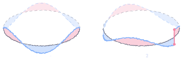
$\frac{m^2}{\sin^2\theta}$ is a centrifugal barrier: winding around a small ring near a pole costs more than winding around the equator. So $P_{\ell}^{|m|}(\cos\theta)\propto\sin^{|m|}\theta$ vanishes at the poles, which single-valuedness demands anyway (every $\psi$ is the same point there). This is the coupling hiding in $\hat{D}_m$’s subscript: $\hat{W}$ lives in the $\theta$ slot, but its $m^2$ comes from the $\psi$ slot.
The floor: $\left<-\hat{A}\right>\geq0$ and $\frac{1}{\sin^2\theta}\geq1\implies\left<\hat{W}\right>\geq1$, so $\ell(\ell+1)\geq m^2\implies\ell\geq|m|$. Winding $m$ times around $z$ costs at least that much curvature.
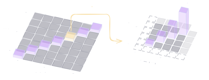
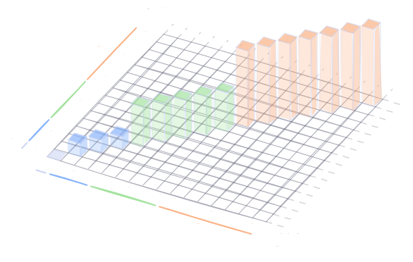
Left is by block (how we diagonalized); right is by eigenvalue (how it’s usually written). Each $\ell$-shell holds $2\ell+1$ degenerate modes: rotations about $x$ and $y$ shuffle the $m$’s within a shell without changing $\hat{\Lambda}$.
References
R. L. Herman, An Introduction to Mathematical Physics via Oscillations, Chapter 9, “Oscillations in Higher Dimensions,” University of North Carolina Wilmington (2012). PDF, licensed CC BY-NC-SA 3.0.
We have fully diagonalized $\hat{\Lambda}$, one slot at a time. Next time, we will see what this says about our basis, work out how to actually find the coefficients $c_{\ell m}$ of any $f$, and use them to solve Laplace’s equation on a sphere.